Outline Optimization Unconstrained Optimization Problems Machine - - PowerPoint PPT Presentation

Optimization

Machine Learning and Pattern Recognition Chris Williams

School of Informatics, University of Edinburgh

October 2014

(These slides have been adapted from previous versions by Charles Sutton, Amos Storkey, David Barber, and from Sam Roweis (1972-2010))

1 / 32

Outline

◮ Unconstrained Optimization Problems

◮ Gradient descent ◮ Second order methods

◮ Constrained Optimization Problems

◮ Linear programming ◮ Quadratic programming

◮ Non-convexity ◮ Reading: Murphy 8.3.2, 8.3.3, 8.5.2.3, 7.3.3.

Barber A.3, A.4, A.5 up to end A.5.1, A.5.7, 17.4.1 pp 379-381.

2 / 32

Why Numerical Optimization?

◮ Logistic regression and neural networks both result in

likelihoods that we cannot maximize in closed form.

◮ End result: an “error function” E(w) which we want to

minimize.

◮ Note argminf(x) = argmax − f(x) ◮ e.g., E(w) can be the negative of the log likelihood. ◮ Consider a fixed training set; think in weight (not input)

• space. At each setting of the weights there is some error

(given the fixed training set): this defines an error surface in weight space.

◮ Learning ≡ descending the error surface.

E(w) E w wj wi E(w)

3 / 32

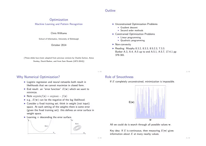
Role of Smoothness

If E completely unconstrained, minimization is impossible. w E(w) All we could do is search through all possible values w. Key idea: If E is continuous, then measuring E(w) gives information about E at many nearby values.

4 / 32

Role of Derivatives

◮ Another powerful tool that we have is the gradient

∇E = ( ∂E ∂w1 , ∂E ∂w2 , . . . , ∂E ∂wD )T .

◮ Two ways to think of this:

◮ Each

∂E ∂wk says: If we wiggle wk and keep everything else the

same, does the error get better or worse?

◮ The function

f(w) = E(w0) + (w − w0)⊤∇E|w0 is a linear function of w that approximates E well in a neighbourhood around w0. (Taylor’s theorem)

◮ Gradient points in the direction of steepest error ascent in

weight space.

5 / 32

Numerical Optimization Algorithms

◮ Numerical optimization algorithms try to solve the general

problem min

w E(w) ◮ Different types of optimization algorithms expect different

inputs

◮ Zero-th order: Requires only a procedure that computes E(w).

These are basically search algorithms.

◮ First order: Also requires the gradient ∇E ◮ Second order: Also requires the Hessian matrix ∇∇E ◮ High order: Uses higher order derivatives. Rarely useful. ◮ Constrained optimization: Only a subset of w values are legal.

◮ Today we’ll discuss first order, second order, and constrained

• ptimization

6 / 32

Optimization Algorithm Cartoon

◮ Basically, numerical optimization algorithms are iterative.

They generate a sequence of points w0, w1, w2, . . . E(w0), E(w1), E(w2), . . . ∇E(w0), ∇E(w1), ∇E(w2), . . .

◮ Basic optimization algorithm is

initialize w while E(w) is unacceptably high calculate g = ∇E Compute direction d from w, E(w), g (can use previous gradients as well...) w ← w − η d end while return w

7 / 32

Gradient Descent

◮ Locally the direction of steepest descent is the gradient. ◮ Simple gradient descent algorithm:

initialize w while E(w) is unacceptably high calculate g ← ∂E

∂w

w ← w − η g end while return w

◮ η is known as the step size (sometimes called learning rate)

◮ We must choose η > 0. ◮ η too small → too slow ◮ η too large → instability 8 / 32

Effect of Step Size

Goal: Minimize E(w) = w2

E(w) = w

−3 −2 −1 1 2 3 2 4 6 8 w E(w)

◮ Take η = 0.1. Works well.

w0 = 1.0 w1 = w0 − 0.1 · 2w0 = 0.8 w2 = w1 − 0.1 · 2w1 = 0.64 w3 = w2 − 0.1 · 2w2 = 0.512 · · · w25 = 0.0047

9 / 32

Effect of Step Size

Goal: Minimize E(w) = w2

E(w) = w

−3 −2 −1 1 2 3 2 4 6 8 w E(w)

◮ Take η = 1.1. Not so good. If you

step too far, you can leap over the region that contains the minimum w0 = 1.0 w1 = w0 − 1.1 · 2w0 = −1.2 w2 = w1 − 1.1 · 2w1 = 1.44 w3 = w2 − 1.1 · 2w2 = −1.72 · · · w25 = 79.50

◮ Finally, take η = 0.000001. What

happens here?

10 / 32

Batch vs online

◮ So far all the objective functions we have seen look like:

E(w; D) =

n

• n=1

En(w; yn, xn). D = {(x1, y1), (x2, y2), . . . (xn, yn)} is the training set.

◮ Each term sum depends on only one training instance ◮ The gradient in this case is always

∂E ∂w =

N

• n=1

∂En ∂w

◮ The algorithm on slide 8 scans all the training instances

before changing the parameters.

◮ Seems dumb if we have millions of training instances. Surely

we can get a gradient that is “good enough” from fewer instances, e.g., a couple thousand? Or maybe even from just

• ne?

11 / 32

Batch vs online

◮ Batch learning: use all patterns in training set, and update

weights after calculating ∂E ∂w =

N

• n=1

∂En ∂w

◮ On-line learning: adapt weights after each pattern

presentation, using ∂En

∂w ◮ Batch more powerful optimization methods ◮ Batch easier to analyze ◮ On-line more feasible for huge or continually growing datasets ◮ On-line may have ability to jump over local optima

12 / 32

Algorithms for Batch Gradient Descent

◮ Here is batch gradient descent.

initialize w while E(w) is unacceptably high calculate g ← N

n=1 ∂En ∂w

w ← w − η g end while return w

◮ This is just the algorithm we have seen before. We have just

“substituted in” the fact that E = N

n=1 En.

13 / 32

Algorithms for Online Gradient Descent

◮ Here is (a particular type of) online gradient descent algorithm

initialize w while E(w) is unacceptably high Pick j as uniform random integer in 1 . . . N calculate g ← ∂Ej

∂w

w ← w − η g end while return w

◮ This version is also called “stochastic gradient ascent”

because we have picked the training instance randomly.

◮ There are other variants of online gradient descent.

14 / 32

Problems With Gradient Descent

◮ Setting the step size η ◮ Shallow valleys ◮ Highly curved error surfaces ◮ Local minima

15 / 32

Shallow Valleys

◮ Typical gradient descent can be fooled in several ways, which

is why more sophisticated methods are used when possible. One problem:

quickly down the valley walls but very slowly along the valley bottom. dE dw

◮ Gradient descent goes very slowly once it hits the shallow

valley.

◮ One hack to deal with this is momentum

dt = βdt−1 + (1 − β)η∇E(wt)

◮ Now you have to set both η and β. Can be difficult and

irritating.

16 / 32

Curved Error Surfaces

◮ A second problem with gradient descent is that the gradient

might not point towards the optimum. This is because of curvature directly at the nearest local minimum.

dE dW

◮ Note: gradient is the locally steepest direction. Need not

directly point toward local optimum.

◮ Local curvature is measured by the Hessian matrix:

Hij = ∂2E/∂wiwj.

◮ By the way, do these ellipses remind you of anything?

17 / 32

Second Order Information

◮ Taylor expansion

E(w + δ) ≃ E(w) + δT ∇wE + 1 2δT Hδ where Hij = ∂2E ∂wi∂wj

◮ H is called the Hessian. ◮ If H is positive definite, this models the error surface as a

quadratic bowl.

18 / 32

Quadratic Bowl

−1 1 −1 1 1 2 3

19 / 32

Direct Optimization

◮ A quadratic function

E(w) = 1 2wT Hw + bT w can be minimised directly using w = −H−1b but this requires

◮ Knowing/computing H, which has size O(D2) for a

D-dimensional parameter space

◮ Inverting H, O(D3) 20 / 32

Newton’s Method

◮ Use the second order Taylor expansion

E(w + δ) ≃ E(w) + δT ∇wE + 1 2δT Hδ

◮ From the last slide, the minimum of the approximation is

δ∗ = −H−1∇wE

◮ Use that as the direction in steepest descent ◮ This is called Newton’s method. ◮ You may have heard of Newton’s method for finding a root,

i.e., a point x such that f(x) = 0. Similar thing, we are finding zeros of ∇f.

21 / 32

Advanced First Order Methods

◮ Newton’s method is fast in that once you are close enough to

a minimum.

◮ What we mean by this is that it needs very few iterations to

get close to the optimum (You can actually prove this if you take an optimization course)

◮ If you have a not-too-large number of parameters and

instances, this is probably method of choice.

◮ But for most ML problems, it is slow. Why? How many

second derivatives are there?

◮ Instead we use “fancy” first-order methods that try to

approximate second order information using only gradients.

◮ These are the state of the art for batch methods

◮ One type: Quasi-Newton methods (I like one called limited

memory BFGS).

◮ Conjugate gradient ◮ We won’t discuss how these work, but you should know that

they exist so that you can use them.

22 / 32

Constrained problems

◮ Constraints: e.g. f(w) < 0. ◮ Example: Observe the points {0.5, 1.0} from a Gaussian with

known mean µ = 0.8 and unknown standard deviation σ. Want to estimate σ by maximum likelihood.

◮ Constraint: σ must be positive. ◮ In this case to find the maximum likelihood solution, the

• ptimization problem is

max

σ 2

• i=1

[− 1 2σ2 (xi − µ)2 − 1 2 log(2πσ2)] subject to σ > 0

◮ In this case: solution can be done analytically. More complex

cases require a numerical method for constrained optimization.

23 / 32

Constrained problems

Either remove constraints by re-parameterization. E.g. w > 0. Set φ = log(w). Now φ unconstrained. Or use a constrained optimization method, e.g. for linear programming, quadratic programming.

24 / 32

Linear Programming

◮ Find optimum, within a (potentially unbounded) polytope, of

a linear function

◮ Polytope = polygon or higher dimensional generalization

thereof.

◮ Easy: maximum (if it exists) must be at vertex of polytope (or

• n a convex set containing such a vertex). Hill climb on

vertices using an adjacency walk (Simplex algorithm)

25 / 32

Quadratic Programming

◮ Find optimum, within a (potentially unbounded) polytope, of

a quadratic form

◮ Interior point methods, Active set methods. ◮ Second order methods for convex quadratic functions

Newton-Raphson, Conjugate Gradient variants.

◮ A number of machine learning methods are cast as quadratic

programming problems (e.g. Support Vector Machines).

26 / 32

Non-convexity and local minima

◮ If you follow the gradient, where will you end up? Once you

hit a local minimum, gradient is 0, so you stop.

error parameter space

◮ Certain nice functions, such as the likelihood for linear and

logistic regression are convex, meaning that the second derivative is always positive. This implies that any local minimum is global.

27 / 32

◮ Dealing with local minima: Train multiple models from

different starting places, and then choose best (or combine in some way).

◮ No guarantees. Unrealistic to believe this will find global

mimimum.

◮ Local minima occur, e.g. for neural networks ◮ Bayesian interpretation, where E(w) = − log p(w|D) ◮ Finding local minima of E(w) as a way of approximating

integration over the posterior by finding local maxima of p(w|D)

28 / 32

Convex Functions

◮ A function f : Rd → R is convex if for α ∈ [0, 1]

f(αx + (1 − α)y) ≤ αf(x) + (1 − α)f(y) Essentially “bowl shaped”

◮ Examples:

f(x) = x2 f(x) = − log x f(x) = log

• d

exp{xd}

• ◮ If f differentiable, this implies

f(x0) + (x − x0)⊤∇f|x0 ≤ f(x) for all x and x0. (To see this: take limit of above as x → y.)

◮ This implies that any local minimum is a global one!

29 / 32

Convex Optimization Problems

◮ A convex optimization problem is one that can be written as

min f0(x) subject to fi(x) ≤ 0 i ∈ {1 . . . N} for some choice of functions f0 . . . fN where each fi is convex

◮ Optimise convex function over a convex set... ◮ Unconstrained problems: Use methods from before. You’ll

find a global optimum!

◮ Convexity means any local optimum is also global optimum. ◮ Constrained convex problems: Interior point methods, Active

set methods.

◮ Most convex optimization problems can be solved efficiently in

practice.

◮ (How high a scale you can reach depends on the type of

problem you have)

30 / 32

Optimization: Summary

◮ Complex mathematical area. Do not implement your own

• ptimization algorithms if you can help it!

◮ My advice: For unconstrained problems

◮ Batch is less hassle than online. But if you have big data, you

must use online. Batch is too slow

◮ (For neural networks, typically online methods are method of

choice.)

◮ If online, you use gradient descent. Forget about second order

stuff.

◮ If batch, use one of the fancy first-order methods

(quasi-Newton or conjugate gradients). DO NOT implement either of these yourself!

◮ If you have a constrained problem

◮ Linear programs are easy. Use off the shelf tools. ◮ More than that: Try to convert into unconstrained problem.

◮ Convex problems: Global minimum. Non-convex: Local

• ptima.

31 / 32

What you should take away

◮ Complex mathematical area. Do not implement your own

• ptimization algorithms if you can help it!

◮ Stuff you should understand:

◮ How and why we convert learning problems into optimization

problems

◮ Modularity between modelling and optimization ◮ Gradient descent ◮ Why gradient descent can run into problems ◮ Especially local minima

◮ Methods of choice: Fancy first-order methods (e.g.,

quasi-Newton, CG) for moderate amounts of data. Stochastic gradient for large amounts of data.

32 / 32