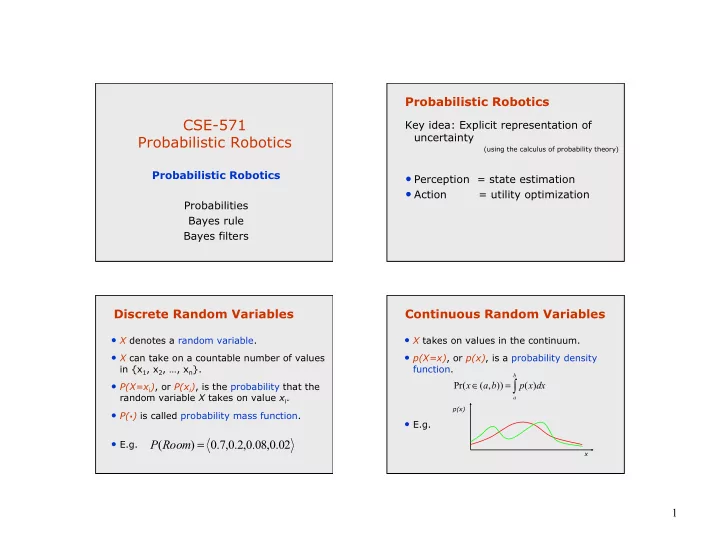
P(X=x i ) , or P(x i ) , is the probability that the = Pr( x - PowerPoint PPT Presentation

Probabilistic Robotics CSE-571 Key idea: Explicit representation of uncertainty Probabilistic Robotics (using the calculus of probability theory) Probabilistic Robotics • Perception = state estimation • Action = utility optimization Probabilities Bayes rule Bayes filters Discrete Random Variables Continuous Random Variables • X denotes a random variable. • X takes on values in the continuum. • X can take on a countable number of values • p(X=x) , or p(x) , is a probability density in {x 1 , x 2 , …, x n }. function. b ∫ • P(X=x i ) , or P(x i ) , is the probability that the ∈ = Pr( x ( a , b )) p ( x ) dx random variable X takes on value x i . a p(x) • P( ) is called probability mass function. . • E.g. = • E.g. P ( Room ) 0 . 7 , 0 . 2 , 0 . 08 , 0 . 02 x 1

Joint and Conditional Probability Law of Total Probability, Marginals • P(X=x and Y=y) = P(x,y) Discrete case Continuous case • If X and Y are independent then ∑ P x = ∫ p x dx = ( ) 1 ( ) 1 P(x,y) = P(x) P(y) x • P(x | y) is the probability of x given y ∑ = ∫ = P ( x ) P ( x , y ) p ( x ) p ( x , y ) dy P(x | y) = P(x,y) / P(y) y P(x,y) = P(x | y) P(y) ∑ ∫ = • If X and Y are independent then P ( x ) P ( x | y ) P ( y ) = p ( x ) p ( x | y ) p ( y ) dy y P(x | y) = P(x) Bayes Formula Normalization = = P ( x , y ) P ( x | y ) P ( y ) P ( y | x ) P ( x ) ⇒ P y x P x ( | ) ( ) = = η P x y ( ) P y x P x ( | ) ( ) P y ( ) ⋅ P ( y | x ) P ( x ) likelihood prior = = P ( x y ) = ∑ 1 η = − 1 P y ( ) P ( y ) evidence P y x P x ( | ') ( ') x ' • Often causal knowledge is easier to obtain than diagnostic knowledge. • Bayes rule allows us to use causal knowledge. 2

Example Simple Example of State Estimation • Suppose a robot obtains measurement z P ( z | open ) = 0.6 P ( z | ¬ open ) = 0.3 • What is P(open|z)? P ( open ) = P ( ¬ open ) = 0.5 P ( z | open ) P ( open ) = P ( open | z ) + ¬ ¬ P ( z | open ) p ( open ) P ( z | open ) p ( open ) ⋅ 0 . 6 0 . 5 2 = = = P ( open | z ) 0 . 67 ⋅ + ⋅ 0 . 6 0 . 5 0 . 3 0 . 5 3 • z raises the probability that the door is open. Normalization Conditioning P y x P x ( | ) ( ) = = η P x y ( ) P y x P x ( | ) ( ) • Bayes rule and background knowledge: P y ( ) P ( y | x , z ) P ( x | z ) = ∑ 1 − = η = 1 P ( x | y , z ) P y ( ) P y x P x ( | ') ( ') P ( y | z ) x ' Algorithm: ∀ = x : aux P ( y | x ) P ( x ) ? x | y ∫ = P ( x y ) P ( x | y , z ) P ( z ) dz 1 η = ∑ ? aux ∫ = P ( x | y , z ) P ( z | y ) dz x | y x ∀ = η x : P ( x | y ) aux ? x | y ∫ = P ( x | y , z ) P ( y | z ) dz 3

Conditioning Conditional Independence • Bayes rule and background knowledge: = P ( x , y z ) P ( x | z ) P ( y | z ) P ( y | x , z ) P ( x | z ) = P ( x | y , z ) P ( y | z ) • Equivalent to = P ( x z ) P ( x | z , y ) and = ∫ P x y ( ) P x y z P z y dz ( | , ) ( | ) = P ( y z ) P ( y | z , x ) Recursive Bayesian Updating Simple Example of State Estimation • Suppose our robot obtains another P ( z | x , z , … , z ) P ( x | z , … , z ) − − n 1 n 1 1 n 1 = P ( x | z , … , z ) 1 n observation z 2 . P ( z | z , … , z ) − n 1 n 1 • What is P(open| z 1, z 2 )? Markov assumption : z n is conditionally independent of z 1 ,...,z n-1 given x. P ( x | z 1 , … , z n ) = P ( z n | x ) P ( x | z 1 , … , z n − 1 ) P ( z n | z 1 , … , z n − 1 ) = η P ( z n | x ) P ( x | z 1 , … , z n − 1 ) ∏ = η 1... n P ( z i | x ) P ( x ) i = 1... n 4

Bayes Filters: Framework Example: Second Measurement • Given: P ( z 2 | open ) = 0.5 P ( z 2 | ¬ open ) = 0.6 • Stream of observations z and action data u: P ( open | z 1 ) = 2 / 3 P ( ¬ open | z 1 ) = 1/ 3 = d { u , z … , u , z } − t 1 2 t 1 t • Sensor model P(z|x). P ( z | open ) P ( open | z ) = P ( open | z , z ) 2 1 • Action model P(x|u,x ’ ) . 2 1 P ( z | open ) P ( open | z ) + P ( z | ¬ open ) P ( ¬ open | z ) 2 1 2 1 • Prior probability of the system state P(x). 1 2 ⋅ • Wanted: 5 2 3 = = = 0 . 625 1 2 3 1 8 • Estimate of the state X of a dynamical system. ⋅ + ⋅ 2 3 5 3 • The posterior of the state is also called Belief : = • z 2 lowers the probability that the door is open. Bel ( x ) P ( x | u , z … , u , z ) − t t 1 2 t 1 t z = observation Bayes Filter Algorithm ∫ u = action = η Bayes Filters Bel ( x ) P ( z | x ) P ( x | u , x ) Bel ( x ) dx x = state − − − t t t t t t 1 t 1 t 1 Algorithm Bayes_filter ( Bel(x),d ): = 1. Bel ( x ) P ( x | u , z … , u , z ) t t 1 1 t t 2. n = 0 = η P ( z | x , u , z , … , u ) P ( x | u , z , … , u ) 3. If d is a perceptual data item z then Bayes t t 1 1 t t 1 1 t 4. For all x do = η P ( z | x ) P ( x | u , z , … , u ) = Bel ' ( x ) P ( z | x ) Bel ( x ) Markov 5. t t t 1 1 t η = η + Bel ' x ( ) 6. Total prob. 7. For all x do ∫ = η P ( z t | x t ) P ( x t | u 1 , z 1 , … , u t , x t − 1 ) P ( x t − 1 | u 1 , z 1 , … , u t ) dx t − 1 − = η 1 8. Bel ' ( x ) Bel ' ( x ) 9. Else if d is an action data item u then ∫ = η P ( z | x ) P ( x | u , x ) P ( x | u , z , … , u ) dx Markov t t t t t − 1 t − 1 1 1 t t − 1 10. For all x do ∫ Bel '( x ) = 11. P ( x | u , x ') Bel ( x ') dx ' ∫ = η P ( z | x ) P ( x | u , x ) Bel ( x ) dx t t t t t − 1 t − 1 t − 1 12. Return Bel ’ (x) 5

Markov Assumption Dynamic Environments • Two possible locations x 1 and x 2 • P(x 1 )=0.99 • P(z| x 2 )=0.09 P(z| x 1 )=0.07 1 = p ( z | x , z , u ) p ( z | x ) p(x2 | d) p(x1 | d) 0.9 − t 0 : t 1 : t 1 1 : t t t 0.8 = p ( x | x , z , u ) p ( x | x , u ) 0.7 − − − t 1 : t 1 1 : t 1 1 : t t t 1 t 0.6 p( x | d) Underlying Assumptions 0.5 0.4 • Static world 0.3 • Independent noise 0.2 0.1 • Perfect model, no approximation errors 0 5 10 15 20 25 30 35 40 45 50 Number of integrations Representations for Bayesian Robot Localization Kalman filters (late-80s) • Gaussians, unimodal Discrete approaches ( ’ 95) • approximately linear models • Topological representation ( ’ 95) • position tracking • uncertainty handling (POMDPs) • occas. global localization, recovery Bayes Filters for • Grid-based, metric representation ( ’ 96) Robot Localization • global localization, recovery Robotics AI Particle filters ( ’ 99) Multi-hypothesis ( ’ 00) • sample-based representation • multiple Kalman filters • global localization, recovery • global localization, recovery 6

Bayes Filters are Familiar! Summary • Bayes rule allows us to compute ∫ = η Bel ( x ) P ( z | x ) P ( x | u , x ) Bel ( x ) dx − − − t t t t t t 1 t 1 t 1 probabilities that are hard to assess otherwise. • Kalman filters • Under the Markov assumption, • Particle filters recursive Bayesian updating can be • Hidden Markov models used to efficiently combine evidence. • Dynamic Bayesian networks • Bayes filters are a probabilistic tool • Partially Observable Markov Decision Processes (POMDPs) for estimating the state of dynamic systems. 7