Outline of the talk Nuclear Magnetic Resonance in ferromagnets: - - PowerPoint PPT Presentation

outline of the talk
SMART_READER_LITE
LIVE PREVIEW

Outline of the talk Nuclear Magnetic Resonance in ferromagnets: - - PowerPoint PPT Presentation

Outline of the talk Nuclear Magnetic Resonance in ferromagnets: NMR in ferromagnets: an analysis tool among others Basis of Nuclear Magnetic Resonance structural and magnetic properties investigations Quantum description


slide-1
SLIDE 1

Nuclear Magnetic Resonance in ferromagnets: structural and magnetic properties investigations

Christian MENY

Institut de Physique et Chimie des Matériaux de Strasbourg UMR 7504 ULP-ECPM-CNRS, BP 43, 23 rue du Loess, 67034 Strasbourg Cedex 2, France Tel : +33 388 107 007 Email : Christrian.meny@ipcms.unistra.fr

Outline of the talk

  • NMR in ferromagnets: an analysis tool among others
  • Basis of Nuclear Magnetic Resonance

– Quantum description – Classical description – Spin Echo

  • Particularities of NMR in ferromagnets
  • Structural information by NMR
  • Local symmetry
  • Local chemical environment
  • Magnetic information by NMR
  • Hyperfine field profile
  • Field and temperature dependent measurements
  • Local magnetic susceptibility: 3D NMR in Ferromagnets
  • Restoring field
  • Magnetization reversal inhomogeneity
  • Magnetic anisotropy inhomogeneity
  • Conclusion

NMR in ferromagnets: an analysis tool among others

  • Free surface

– Electron Diffraction : RHEED, LEED: Growth mode, 2D Surface structure, Orientations – Auger Spectroscopy : AES: Growth mode, Surface diffusion & segregation – Imaging : STM, AFM: Direct topological view

  • Volume

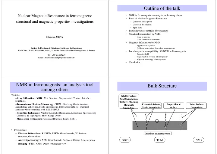
–Xray Diffraction : XRD : Xtal Structure, Super-period, Texture, Interface roughness –Transmission Electron Microscopy : TEM : Stacking, Grain structure, Superlattice coherence, Misfit dislocations, Interface roughness, chemical analyses when combined with EELS/EDXS –Hyperfine techniques: Nuclear Magnetic Resonance, Mössbauer Spectroscopy : Chemical & Topological Short Range Order –Many other techniques: Neutron diffraction, Exafs, RBS…

Bulk Structure

Xtal Structure Xtal Orientation Texture, Stacking Mosaicity Grain Size Impurities at defects Interface nanostructure Extended defects, Grain boundaries Point Defects, Impurities

XRD NMR TEM

slide-2
SLIDE 2

Interface Structure

Long Range Roughness Interface Compound Alloyed Interface Dislocations

XRD Surface AFM STM AES LEED RHEED TEM NMR

Outline of the talk

  • NMR in ferromagnets: an analysis tool among others
  • Basis of Nuclear Magnetic Resonance

– Quantum description – Classical description – Spin Echo

  • Particularities of NMR in ferromagnets
  • Structural information by NMR
  • Local symmetry
  • Local chemical environment
  • Magnetic information by NMR
  • Hyperfine field profile
  • Field and temperature dependent measurements
  • Local magnetic susceptibility: 3D NMR in Ferromagnets
  • Restoring field
  • Magnetization reversal inhomogeneity
  • Magnetic anisotropy inhomogeneity
  • Conclusion
  • Quantum mechanics: Resonant

Absorption of Photon

Basis of Nuclear Magnetic Resonance

Spin 1/2 H0 = 0 L Photon H1() 1/2 1/2 H0  0 Resonance: L H0: Static magnetic field: Zeeman Effect H1: Radiofrequency field : Resonant Absorption

Basis of Nuclear Magnetic Resonance

  • Characteristics of nuclei:

– Spin

  • Has to be non zero :from ½ (1H) to 7 (176Lu)

– Odd number of neutrons or protons

– gyromagnetic ratio 

  • The ratio of magnetic dipole moment to the angular momentum

– M=L – Characterizes the motion in a magnetic field

slide-3
SLIDE 3

Observable Elements & Sensitivity

In practice:

Organic materials: H, F, P (17O, 4N, 13C) Metalloids: Ga, B, As, In (Si, Se, Te) Normal metals: Li, Na, Al (Be, K) Transition Metals: V, Mn, Co, Cu, Nb, La, Re (Y, Pt, Ta) Rare Earths: Pr, Eu, Tb, Ho (Nd, Gd) H He Li Be B C N O F Ne Na Mg Al Si P S Cl Ar K Ca Sc Ti V Cr Mn Fe Co Ni Cu Zn Ga Ge As Se Br Kr Rb Sr Y Zr Nb Mo Tc Ru Rh Pd Ag Cd In Sn Sb Te I Xe Cs Ba La Hf Ta W Re Os Ir Pt Au Hg Tl Pb Bi Po At Rn Ce Pr Nd Pm Sm Eu Gd Tb Dy Ho Er Tm Yb Lu Medium Good Bad No

To increase sensitivity:

Low Temperature : NMR signal increases as 1/T (Curie law) High Field : NMR signal increases as 2 =2H2

  • NMR signal can be obtained for all nuclei with non zero nuclear spin

Outline of the talk

  • NMR in ferromagnets: an analysis tool among others
  • Basis of Nuclear Magnetic Resonance

– Quantum description – Classical description – Spin Echo

  • Particularities of NMR in ferromagnets
  • Structural information by NMR
  • Local symmetry
  • Local chemical environment
  • Magnetic information by NMR
  • Hyperfine field profile
  • Field and temperature dependent measurements
  • Local magnetic susceptibility: 3D NMR in Ferromagnets
  • Restoring field
  • Magnetization reversal inhomogeneity
  • Magnetic anisotropy inhomogeneity
  • Conclusion
  • Why is it possible to use a classical description.

– NMR measurements are done simultaneously on a very large number of nuclei

  • NMR processes much easier to explain

NMR Classical description

  • We consider a particle moving about an axis
  • The Newton’s second law:
  • If we multiply both sides by the cross product with the position vector

r we obtain:

 dt p d F  

   

          dt p r d dt p d r dt p d r F r dt p d r F r ) (              

Motion of a particle rotating about an axis

slide-4
SLIDE 4

Motion of an object rotating about an axis

Is called the angular momentum of the particle So we can write: The sum of the torques is equal to the time derivative of the angular momentum. This is the rotational analog of the Newton’s second law

p r L     

 dt L d   

The case of a nuclear spin

Now a consider a nuclear spin of magnetic moment M in a magnetic field From the magnetic field results a torque: And its magnetic moment is defined through is gyromagnetic ratio M=L So the spin equation of motion becomes

H M      

dt M d H M dt L d        

 

Motion of an object rotating about an axis The case of a nuclear spin

The direction of the motion is perpendicular to the plan defined by M and H This is a precession motion.

dt M d H M      

Motion of an object rotating about an axis The case of a nuclear spin

  • Classical view point: Nuclear Precession

H0

dM/dt = MH

slide-5
SLIDE 5
  • How to give a classical description
  • f this quantum process?

NMR Classical description

Spin 1/2 H0 = 0 L Photon H1() 1/2 1/2 H0  0 Resonance: L We need to consider 2 fields: H0: Static magnetic field: Zeeman Effect (OK with what we know) H1: Radiofrequency field : Resonant Absorption ???????

NMR Classical description

  • A rf field is the sum of 2 fields rotating in
  • pposite directions

NMR - Macroscopic Viewpoint

Laboratory frame Rotating frame (L) Rotating frame (L) MnL H0 x y z

In a frame rotating at the same angular velocity L as the spin , the spin looks static. In the frame rotating at velocity L the apparent static magnetic field is ZERO

Mn is Static H’0=0 x y z MnL  H’0 = H0 -  x y

NMR - Macroscopic Viewpoint

Laboratory frame Rotating frame ()

MnL H0 x y z H1

Pulsed H1

Pulse Duration:  Turn Angle:  Particular Turn Angles 2 : MnH0  : Mn Reversal

Mne H0 -  He H1 Z X Y L Off - Resonance Y Mn H1 X Z L At Resonance H0 - 

slide-6
SLIDE 6

NMR - Macroscopic Viewpoint

What is the NMR signal? The component of the nuclear magnetization in the xy plane NMR signal is maximum when the turning angle is 2 A way to measure the NMR signal : Spin Echo

NMR - Macroscopic Viewpoint

Classical (Hahn) Spin Echo Pulse Sequence 

Dephasing (Spread of L)

Mn H1 X Z

Y Mn X

Fast Slow Fast Slow

Y

Y Mn X

Slow Fast

Rotating Frame View - XY Plane

M R E V E R S A L Rephasing Dephasing

H1on 90° t  d



d H1on 180° Spin Echo Free Induction Decay

Pulsed NMR Setup

Sample coil Magnet (H scan) RF pulse (µS) 1 to 1000 MHz (scan) NMR Induction Signal Emission Absorption

Transmitter Receiver t Free Induction Decay in Time Domain Fourier transform NMR FID or Spin Echo integral intensity in Frequency Domain H or  Field or Frequency Scan NMR

NMR – Relaxation times

  • After a spin echo; the spin system has to go back to

equilibrium:

  • 2 relaxation processes:
  • vanishing of the nuclear magnetization in the xy

plane

  • Reorientation of the magnetization towards the Z

axis. Relaxation along the laboratory Z direction: spin lattice relaxation time T1 (10 ms) Relaxation into the xy plane : spin-spin relaxation time T2 (10 s)

slide-7
SLIDE 7

Outline of the talk

  • NMR in ferromagnets: an analysis tool among others
  • Basis of Nuclear Magnetic Resonance

– Quantum description – Classical description – Spin Echo

  • Particularities of NMR in ferromagnets
  • Structural information by NMR
  • Local symmetry
  • Local chemical environment
  • Magnetic information by NMR
  • Hyperfine field profile
  • Field and temperature dependent measurements
  • Local magnetic susceptibility: 3D NMR in Ferromagnets
  • Restoring field
  • Magnetization reversal inhomogeneity
  • Magnetic anisotropy inhomogeneity
  • Conclusion

NMR in ferromagnets: Particularities

  • In ferromagnets the magnetic field H0 is the field inside the material on the

nuclei sites (For example 20 Tesla for Cobalt nuclei in bulk Co).

  • It is called the Hyperfine Field (HF)
  • The HF strength depends on the local symmetry and local chemical

environment of the probed nuclei

Spin 1/2 H0 = 0 L Photon H1() 1/2 1/2 H0 HF Resonance: L

  • An NMR spectrum in a ferromagnet is measured by frequency sweeps
  • it is a number of atoms versus a resonance frequency.
  • Among the “traditional” ferromagnets (Fe, Co and Ni),
  • Co has the highest sensitivity (104 time larger than Fe for example)

Outline of the talk

  • NMR in ferromagnets: an analysis tool among others
  • Basis of Nuclear Magnetic Resonance

– Quantum description – Classical description – Spin Echo

  • Particularities of NMR in ferromagnets
  • Structural information by NMR
  • Local symmetry
  • Local chemical environment
  • Magnetic information by NMR
  • Hyperfine field profile
  • Field and temperature dependent measurements
  • Local magnetic susceptibility: 3D NMR in Ferromagnets
  • Restoring field
  • Magnetization reversal inhomogeneity
  • Magnetic anisotropy inhomogeneity
  • Conclusion

NMR Frequency and Local symmetry: Bulk Co

Spin Echo Intensity

210 215 220 225 230

Frequency (MHz)

Stacking faults hcp Cobalt fcc Cobalt

FCC Dominant

210 215 220 225 230

Frequency (MHz)

Stacking faults hcp Cobalt fcc Cobalt

HCP Dominant

x5 Pure samples: Frequency is the fingerprint of the atom site local symmetry

slide-8
SLIDE 8

Standard - Bulk Cobalt - fcc & hcp

  • fcc base
  • ABCABCABCABC
  • cccccccccccc
  • ABCABCBACBAC
  • ccccchcccccc
  • ABCABCBCABCA
  • ccccchhccccc
  • ABCABCBCBABC
  • ccccchhhcccc
  • hcp base
  • ABABABABABAB
  • hhhhhhhhhhhh
  • ABABACBCBCBC
  • hhhhhchhhhhh
  • ABABACBABABA
  • hhhhhcchhhhh
  • ABABACBACACA
  • hhhhhccchhhh

Perfect 1 fault 2 faults h in c / c in h

Stacking faults in fcc/hcp structures

(111) (001) Bulk Structure of electrodeposited Co Thin Films Quantitative analysis

20 40 60 80 100 1000 2000 3000 4000 5000

fcc fraction hcp fraction 3% 30% Stacking faults:

Volume Fracion (%) Layer Thickness (Å)

Electrodeposited on very flat Au film Initial growth mostly hcp (<20%fcc) Then fcc + SF AFM Imaging: Change of structure correlated to change of film morphology: First stage: flat layers Second stage : Columns

Outline of the talk

  • NMR in ferromagnets: an analysis tool among others
  • Basis of Nuclear Magnetic Resonance

– Quantum description – Classical description – Spin Echo

  • Particularities of NMR in ferromagnets
  • Structural information by NMR
  • Local symmetry
  • Local chemical environment
  • Magnetic information by NMR
  • Hyperfine field profile
  • Field and temperature dependent measurements
  • Local magnetic susceptibility: 3D NMR in Ferromagnets
  • Restoring field
  • Magnetization reversal inhomogeneity
  • Magnetic anisotropy inhomogeneity
  • Conclusion

NMR frequency and Chemical environment

200 220 240 260 50 100 150 200 250

Spin Echo Intensity

100 150 200 250

Co0.90Cu0.10

Frequency (MHz)

0 Cu nn 1 Cu nn 2 Cu nn 2 Ru nn 1 Ru nn 0 Ru nn

Frequency (MHz)

Co0.90Ru0.10

3 Ru nn

Frequency (MHz)

Co0.90Fe0.10

1 Fe nn 2 Fe nn 0 Fe nn 3 Fe nn

  • Alien atoms as nearest neighbor of the probed atom shifts the resonance frequency.

The value and sign of the shift depends on the nature of the neighboring atom. (Cu: -16 MHz; Ru:-25 MHz; Fe: +10 MHz)

slide-9
SLIDE 9

NMR frequency and Chemical environment : quantitative analysis

Decomposition of NMR spectrum with Gaussian lines. NMR intensity increase as 1 NN : grows as C, 2 NN : grows as C2, 3 NN : grows as C3, C: Concentration in alien atoms Random distribution of the alien atoms among the nearest neighbors (NN) of Co. The line intensity follows a binomial law 40 80 120 160 200 240

Frequency (MHz) Spin Echo Intensity

0 Cr nn 2 Cr nn 4 Cr nn 1 Cr nn 3 Cr nn

Co0.86Cr0.14 Co0.96Cr0.04

0 Cr nn 1 Cr nn 2 Cr nn

CoCr: Trend towards segregation at low concentration CoCu: Strong trend towards segregation (immiscible elements) CoFe: Close to solid solution CoRu: Perfect solid solution

Relative line intensities (0, 1, 2, 3 NN) & binomial probability law (Random site occupancy)

NMR frequency and Chemical environment : quantitative analysis

1.0 0.8 0.6 0.4 0.2 0.0 0.8 0.6 0.4 0.2 0.0 0.8 0.6 0.4 0.2 0.0 0.8 0.6 0.4 0.2 0.0 0 5 10 15

Impurity Content (%) Co Ru Co Fe Co Cu Co Cr

Configuration Probability

Problem - Bulk Not Understood

CoPt alloys:

– 2 sets of satellites

  • narrow upwards
  • broad downwards

– Related to position of the nearest neighbor among the 12 NN ? – Long range interactions between Pt impurities ? – Second neighbor shell ?

150 175 200 225 250

Frequency (MHz) Spin Echo Intensity

CoPt0.10 CoPt0.06 CoPt0.02

Frequency Shifts in Co based Alloys

Note * In anisotropic hcp alloys, the shift value depends whether the impurity neighbor is in the same (001) plane as the Co atom or in the adjacent planes: Two satellites ( low & high) are observed for very diluted alloys. In more concentrated alloys (>2%) the two satellites merge into an average one (av) because of the broadening due to long range disorder.

Frequency shift due to impurities in the nearest neighbor shell Nearly proportional to the number of impurities

Impurity Al Si Ti V Cr Mn Fe Ni Cu Ge Nb Ru Re Rh fcc

  • 22
  • 16
  • 40
  • 40
  • 37

+9

  • 7
  • 16
  • 16
  • 47

Phase bcc

Frequency Shift /

  • Imp. NN (MHz)

Frequency Shift /

  • Imp. NN (MHz)

+11

  • 32
  • 22
  • 41

hcp av* low high

Frequency Shift /

  • Imp. NN (MHz)
  • 32
  • 53
  • 10
  • 17
  • 25
  • 16
  • 27
  • 50

0

slide-10
SLIDE 10

Examples : Magnetic multilayers

  • Frequency fingerprint of Chemical/Xtallographic Environment
  • Frequency Ranges correspond to Different Sample Parts

60 100 140 180 0.0 0.2 0.4 0.6 0.8

Co-X admixture (other mixed planes) Co-X admixture (1st mixed plane) x10 Bulk grain boundaries Perfect 111 interface

Spin Echo Intensity (arbitrary) Frequency (MHz)

210 220 230 240 2 4 6 8

Stacking faults (& hcp Co c) hcp Cobalt Mc fcc Cobalt

Interface spectral range Bulk spectral range

Co/Cu multilayer

.../Cu/Co/Cu/... Interface Spectra

Nearly perfect interface (111). Single satellite line corresponding to Co atoms with 3 Cu neighbors. Traces of Co with 2 Cu neighbors. Excellent multilayered structure. The 3 Cu neighbors line is 30% of the interface spectrum. Sharp interfaces but numerous monoatomic step defects Mixed interfaces with some flatter areas (3 Cu neighbors line resolved). Steep concentration profile. Mixed

  • interfaces. Satellite lines of Co with 1 and 2 Cu

neighbors show the presence of several planes containing a weak Cu concentration (3 to 8 %).

Frequency (MHz)

50 100 150 200 250

Spin Echo Intensity

THO IBM IEF PHI

Modeling of Interface Spectra Monoatomic Step Defects

Simulated Spectra

d=2, l=2 d=2, l=4 d=2, l=2 d=4, l=2 12 1110 9 8 7 6 5 4 3 2 1 0 Number of Alien Nearest Neighbors

Interface Model

Parameters of the model d : Average distance between steps l : Average length of straight parts Application : small roughness

Cross section view

l

Top view of mixed plane

d

Spin Echo Intensity

120 140 160 180 200 220 240

Frequency (MHz)

Ru/Cu8Å/Co24Å/Ag2.4Å/Cu20Å /Ag2.4Å /Co24Å

Average distance between steps: 2.8 at.d. Average straight length: 1.6 at.d.

Cross section view

l

Top view of mixed plane

d

Modeling of Interface Spectra Monoatomic Step Defects

slide-11
SLIDE 11

Modeling of Interface Spectra Diffuse Interface

Cross section view

3 Mixed Planes 6 Mixed Planes 1 Mixed Plane 2 Mixed Planes 3 Mixed Planes 12 1110 9 8 7 6 5 4 3 2 1 0

Number of Alien Nearest Neighbors

Simulated Spectra Interface Model

Parameters of the model Concentrations in each plane (Concentration profile) Example : Linear profile Application: Large admixture >2ML

C1 C2 C3 C4 C5 C6 C7

.../Cr/Co/Cr/... Largely Mixed Interfaces

Last full Co plane 1st mixed plane 2nd mixed plane

Spin Echo Intensity Frequency (MHz)

50 100 150 200 250

[Co16Å/Cr8Å]

Cr concentration at.% Hyprfine Field (% of bulk)

100 75 50 25 100 75 50 25

  • 1 0 1 2 3 4 5

Atomic Layer Index

Co Hyperfine field Cr concentration

Mg/Zr/Co multilayers for applications in optics: Asymmetric Co interfaces

Almost perfect Mg/Co interfaces Mixte Co/Zr interfaces

Outline of the talk

  • NMR in ferromagnets: an analysis tool among others
  • Basis of Nuclear Magnetic Resonance

– Quantum description – Classical description – Spin Echo

  • Particularities of NMR in ferromagnets
  • Structural information by NMR
  • Local symmetry
  • Local chemical environment
  • Magnetic information by NMR
  • Hyperfine field profile
  • Field and temperature dependent measurements
  • Local magnetic susceptibility: 3D NMR in Ferromagnets
  • Restoring field
  • Magnetization reversal inhomogeneity
  • Magnetic anisotropy inhomogeneity
  • Conclusion
slide-12
SLIDE 12

Magnetic information: Hyperfine Field Profile

Interface Model : Concentration profile Side output : Average HF in each atomic plane Average HF an estimate of Co magnetic moment at interfaces

1 2 3 4 5 20 40 60 80 100

Ru Concentration (%) Co Hyperfine Field (% of bulk)

Interface Profiles Interface Plane Index (1: last pure Co)

N M R T h eo ry C R u H F /H F b u lk µ /µ b u lk C R u 1 .0 0 1 .0 0 0 0 .9 9 1 .0 3 0 2 .5 0 .9 4 0 .9 7 0 1 7 0 .7 5 0 .8 9 2 5 5 0 0 .4 0 0 .6 3 5 0 8 2 0 .0 4 0 .1 3 7 5

Frequency (MHz)

50 100 150 200 250

Co /Ru

Bulk Co planes 3rd mixed plane 50%Ru 2nd mixed plane 17%Ru 1st mixed plane 2.5% Ru

Spin Echo Intensity

32Å

MBE Grown

X Multilayers

Theory: D.Stoefler IPCMS

Co clusters in matrices

  • Magnetic properties depends on the size of the clusters:

– Large clusters : multi-domain – Small clusters : single domain and depending on temperature, the magnetic moment direction is blocked (at low temperature) or rotating randomly in any direction (at high temperature)

Low T High T : Super- paramagnetism Domain structure and blocking temperature is determined by the magnetic anisotropy of the material and by the size of the clusters. To understand the magnetic properties we need to know the size (distribution) of the clusters and the magnetic anisotropy

Magnetic Properties by NMR With additional external static magnetic field

210 215 220 225 230

Spin Echo Intensity Frequency (MHz)

External field 0 Oe 500 Oe 1000 Oe 1500 Oe

Tann = 1000°C Texp = 4.2 K

Lower frequency line Large Co clusters, multidomain, fcc :

  • No demagnetizing field (217 MHz)
  • Presence of Bloch walls (no shift in low field)

Upper frequency line Small Co clusters, single domain, fcc :

  • Not hcp, no HF anisotropy (no broadening with Hext)
  • Demagnetizing field -6 kOe (223 MHz)
  • No Bloch wall (shift -Hext from the smallest Hext)

FCC Co ?

Co clusters in Silica

210 220 230 240 Temperature 4.2 K 77 K 300 K

Spin Echo Intensity Frequency (MHz)

Tann = 800°C Hext = 0 Oe When Co Clusters are superparamagnetic: No NMR signal Lower frequency line Large Co clusters ferromagnetic :

  • Constant intensity
  • Upper frequency line

Small Co clusters superparamagnetic

  • Loss of intensity with increasing temperature
  • Large distribution of blocking temperatures

Large distribution of sizes : Coexistence of small single domain clusters and of large multidomain clusters

Magnetic Properties by NMR NMR measurements versus temperature

slide-13
SLIDE 13

Outline of the talk

  • NMR in ferromagnets: an analysis tool among others
  • Basis of Nuclear Magnetic Resonance

– Quantum description – Classical description – Spin Echo

  • Particularities of NMR in ferromagnets
  • Structural information by NMR
  • Local symmetry
  • Local chemical environment
  • Magnetic information by NMR
  • Hyperfine field profile
  • Field and temperature dependent measurements
  • Local magnetic susceptibility: 3D NMR in Ferromagnets
  • Restoring field
  • Magnetization reversal inhomogeneity
  • Magnetic anisotropy inhomogeneity
  • Conclusion

NMR - Macroscopic Viewpoint

Laboratory frame Rotating frame ()

MnL H0 x y z H1

Pulsed H1

Pulse Duration:  Turn Angle:  Particular Turn Angles 2 : MnH0  : Mn Reversal

Mne H0 -  He H1 Z X Y L Off - Resonance Y Mn H1 X Z L At Resonance H0 - 

Measured NMR signal is proportional to the magnitude of the nuclear magnetization in the XY plane: Maximum when turn angle 1= /2

Log(H1)

Hoptimum

Spin Echo Intensity

1/3 1 3

External Static Field H0

10 to 100 kOe

RF Field H1

10 to 100 Oe

Non Magnetic Sample

Bopt = /2

1

Maximum of NMR signal depends only on the properties of the probed Nucleus and on the experimental set up:  is a fixed experimental parameter  : the gyromagnetic ratio of the nucleus

NMR intensity (Spin echo intensity) vs RF field strength

Restoring Field related to :

  • Anisotropy field (single domain behavior)
  • Coercive field (domain nucleation or domain wall stiffness)
  • Exchange bias, Coupling field (coupling energy between layers/grains)

(ferro) H 2 HF/ H

  • pt

res

    

HF: Hyperfine Field

10 to 500 kG

Hr : Restoring Field Excitation B1 = H1: B1/H1 = HF/Hr =  For the maximum NMR intensity: Hr=HF*Hopt(ferro)/Bopt(non ferro) Hr=HF*Hopt(ferro)2/

Magnetic Sample

RF Field H1

0.01 to 1 Oe

µe

RF Field B1=H1

10 to 100 G

Hr HF

1/ Hr Log(H1)

Soft

Log(H1) Spin Echo Intensity 1/ Hr

Hard

 

Enhancement factor & Restoring Field

slide-14
SLIDE 14

210 215 220 225 230 200 400 600 800 1000

Restoring Field (Oe) Frequency (MHz)

3D NMR spectra in ferromagnets

How to visualize inhomogeneities NMR Intensity vs

  • Frequency : StructuralNMR
  • RF Field : Magnetic stiffness

Line

  • f

Crest

Scaled RF Field (Oe)

"Single Xtal" hcp Co

210 215 220 225 230 40 100 200 400

fcc Co Stacking Faults hcp Co Mc Frequency (MHz)

3D Curves

The larger the strength of the H1 field we need to apply, the stiffer the part of the sample under investigation

Outline of the talk

  • NMR in ferromagnets: an analysis tool among others
  • Basis of Nuclear Magnetic Resonance

– Quantum description – Classical description – Spin Echo

  • Particularities of NMR in ferromagnets
  • Structural information by NMR
  • Local symmetry
  • Local chemical environment
  • Magnetic information by NMR
  • Hyperfine field profile
  • Field and temperature dependent measurements
  • Local magnetic susceptibility: 3D NMR in Ferromagnets
  • Restoring field
  • Magnetization reversal inhomogeneity
  • Magnetic anisotropy inhomogeneity
  • Conclusion

From softest

Grain boundaries (small grains) Interface planes Stacking faults (zones of) Bulk hcp (Mc axis) Bulk fcc Bulk hcp (M//c axis)

To hardest

Structure & Magnetic Stiffness

/NiFe/FeMn

22

/Cu Co75 Spin Valve (IBM)

100 120 140 160 180 200 10 20 30 40 50 60 70

Frequency (MHz) Restoring Field (Oe) Spectrum

220

Frequency= environment

  • High frequency, bulk Co : Co

atoms surrounded by other Co atoms

  • The frequency gives the local

symmetry (fcc or hc Co)

  • Low frequency, interface: Co

atoms by Co and Cu atoms Radiofrequency strength vs frequency :

  • shows how magnetically stiff each

environment is Magnetization reversal initiated where the sample is the less stiff

Coupling Oscillations

  • Interface planes partly decoupled from inner planes
  • softer than bulk (usual)
  • more sensitive to AF coupling (expected)
  • AF coupling only partly transferred to inner planes

10 15 20 25 30 35 200 400 600 800 1000 1200 1400

Bulk Hr Interface Hr MR Restoring Field (Oe) Ru Thickness (Å)

0.0 0.2 0.4 0.6 0.8 1.0 1.2

MagnetoResistance Ratio (%)

/Ru Co32Å

X Multilayers

Excitation mode for Ferromagnetic coupling Excitation mode for Anti-Ferromagnetic coupling

slide-15
SLIDE 15

Magnetization Process Homogeneity

Discriminates between

  • Inhomogeneous

magnetization process

And

  • Coherent rotation of a

net remanent magnetization e.g. Biquadratic Coupling Co/Cu Multilayers

Co15ÅCu9Å AF + F coupling Co15ÅCu15Å Ferromagnetic coupling Co10ÅCu10Å Biquadratic coupling ?

180 200 220 1000 300 100 30 180 200 220 1000 300 100 30

Scaled RF Field (Oe)

180 200 220 1000 300 100 30

F r e q u e n c y ( M H z ) M/Ms

  • 8k
  • 4k

4k 8k

  • 1.0
  • 0.5

0.0 0.5 1.0

External field (Oe)

  • 8k
  • 4k

4k 8k

  • 1.0
  • 0.5

0.0 0.5 1.0 M/Ms

External field (Oe)

Inhomogeneities of Co Dispersion, Inhomogeneities of Magnetic Anisotropy: Co clusters in Cu

100 1000 10000 100000

50 100 150 200

Hres, 2

 = 200 MHz

Spin Echo Intensity

Hres, 1

100 1000 10000 100000

100 200 300 400 500 600

Scaled RF Field strength (Oe)

Hres, 2 Hres, 1

 = 215 MHz

Spin Echo Intensity 50 100 150 200

100 200 300 400

experimental spectrum Stif magnetic Co clusters soft magnetic Co alloy Spin Echo Intensity Frequency (MHz)

Spectrum decomposition into two phases with different magnetic anisotropy

Stif : Pure fcc Co clusters + interface Soft : CoCu alloy grains Evidence for the existence of two phases with different magnetic anisotropies

FC ZFC Measurements: 2 different blocking temperatures:

  • Usual interpretation: 2 populations with different typical diameter.
  • The NMR viewpoint:

The ratio of the blocking temperatures equals the ratio

  • f the NMR restoring field:

The cluster size of the two populations is similar but because of their chemical composition their anisotropy is different.

Inhomogeneities of Co Dispersion, Inhomogeneities of Magnetic Anisotropy: Co clusters in Cu

Conclusions

NMR allows to get specific information about of the structural and magnetic properties in different parts of the sample Bulk Co

  • Structure of the bulk of the layers and their respective magnetic stiffness

Small grains lead to soft layers because of an increased number grain boundaries

At interfaces

  • Morphology of the Interfaces
  • Magnetization profile.
  • Magnetic stiffness depends on interface disorder and defects

Between layers

  • Coupling strength
  • Discriminates between coherent and incoherent magnetization process.

In granular systems

  • Distribution of sizes, magnetic anisotropy, superparamagnetism.

Ref:

  • C. MENY, P. PANISSOD

Modern Magnetic Resonance, G. Webb, Ed., Springer, Heidelberg, 2007. and references therein

  • P. PANISSOD, C. MENY
  • Appl. Magn. Reson. 19, 447-460 (2000)