
SLIDE 1
IAML: Optimization
Nigel Goddard School of Informatics Semester 1
1 / 24
Outline
◮ Why we use optimization in machine learning ◮ The general optimization problem ◮ Gradient descent ◮ Problems with gradient descent ◮ Batch versus online ◮ Second-order methods ◮ Constrained optimization
Many illustrations, text, and general ideas from these slides are taken from Sam Roweis (1972-2010). 2 / 24
Why Optimization
◮ A main idea in machine learning is to convert the learning
problem into a continuous optimization problem.
◮ Examples: Linear regression, logistic regression (we have
seen), neural networks, SVMs (we will see these later)
◮ One way to do this is maximum likelihood
ℓ(w) = log p(y1, x1, y2, x2, . . . , yn, xn|w) = log
n
- i=1
p(yi, xi|w) =
n
- i=1
log p(yi, xi|w)
◮ Example: Linear regression
3 / 24
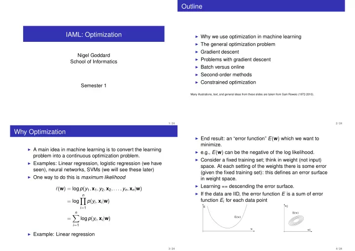
◮ End result: an “error function” E(w) which we want to
minimize.
◮ e.g., E(w) can be the negative of the log likelihood. ◮ Consider a fixed training set; think in weight (not input)
- space. At each setting of the weights there is some error
(given the fixed training set): this defines an error surface in weight space.
◮ Learning == descending the error surface. ◮ If the data are IID, the error function E is a sum of error
function Ei for each data point
E(w) E w wj wi E(w)
4 / 24