In SMV I IAML: Support Vector Machines II We saw: Max margin trick - - PowerPoint PPT Presentation

IAML: Support Vector Machines II

Nigel Goddard School of Informatics Semester 1

1 / 25

In SMV I

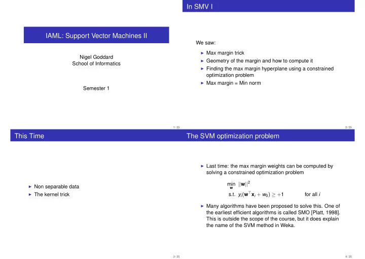
We saw:

◮ Max margin trick ◮ Geometry of the margin and how to compute it ◮ Finding the max margin hyperplane using a constrained

• ptimization problem

◮ Max margin = Min norm

2 / 25

This Time

◮ Non separable data ◮ The kernel trick

3 / 25

The SVM optimization problem

◮ Last time: the max margin weights can be computed by

solving a constrained optimization problem min

w

||w||2 s.t. yi(w⊤xi + w0) ≥ +1 for all i

◮ Many algorithms have been proposed to solve this. One of

the earliest efficient algorithms is called SMO [Platt, 1998]. This is outside the scope of the course, but it does explain the name of the SVM method in Weka.

4 / 25

Finding the optimum

◮ If you go through some advanced maths (Lagrange

multipliers, etc.), it turns out that you can show something

• remarkable. Optimal parameters look like

w =

• i

αiyixi

◮ Furthermore, solution is sparse. Optimal hyperplane is

determined by just a few examples: call these support vectors

5 / 25

Why a solution of this form?

If you move the points not on the marginal hyperplanes, solution doesn’t change - therefore those points don’t matter.

~ x x x x

• margin

w

6 / 25

Finding the optimum

◮ If you go through some advanced maths (Lagrange

multipliers, etc.), it turns out that you can show something

• remarkable. Optimal parameters look like

w =

• i

αiyixi

◮ Furthermore, solution is sparse. Optimal hyperplane is

determined by just a few examples: call these support vectors

◮ αi = 0 for non-support patterns ◮ Optimization problem to find αi has no local minima (like

logistic regression)

◮ Prediction on new data point x

f(x) = sign((w⊤x) + w0) = sign(

n

• i=1

αiyi(x⊤

i x) + w0)

7 / 25

Non-separable training sets

◮ If data set is not linearly separable, the optimization

problem that we have given has no solution. min

w

||w||2 s.t. yi(w⊤xi + w0) ≥ +1 for all i

◮ Why?

8 / 25

Non-separable training sets

◮ If data set is not linearly separable, the optimization

problem that we have given has no solution. min

w

||w||2 s.t. yi(w⊤xi + w0) ≥ +1 for all i

◮ Why? ◮ Solution: Don’t require that we classify all points correctly.

Allow the algorithm to choose to ignore some of the points.

◮ This is obviously dangerous (why not ignore all of them?)

so we need to give it a penalty for doing so.

9 / 25

~

x x x x

• margin
• !

w

10 / 25

Slack

◮ Solution: Add a “slack” variable ξi ≥ 0 for each training

example.

◮ If the slack variable is high, we get to relax the constraint,

but we pay a price

◮ New optimization problem is to minimize

||w||2 + C(

n

• i=1

ξk

i )

subject to the constraints w⊤xi + w0 ≥ 1 − ξi for yi = +1 w⊤xi + w0 ≤ −1 + ξi for yi = −1

◮ Usually set k = 1. C is a trade-off parameter. Large C

gives a large penalty to errors.

◮ Solution has same form, but support vectors also include

all where ξi = 0. Why?

11 / 25

Think about ridge regression again

◮ Our max margin + slack optimization problem is to

minimize: ||w||2 + C(

n

• i=1

ξi)k subject to the constraints w⊤xi + w0 ≥ 1 − ξi for yi = +1 w⊤xi + w0 ≤ −1 + ξi for yi = −1

◮ This looks a even more like ridge regression than the

non-slack problem:

◮ C(n

i=1 ξi)k measures how well we fit the data

◮ ||w||2 penalizes weight vectors with a large norm

◮ So C can be viewed as a regularization parameters, like λ

in ridge regression or regularized logistic regression

◮ You’re allowed to make this tradeoff even when the data

set is separable!

12 / 25

Why you might want slack in a separable data set

x x x x x x x x

• x1

x2 w

x x x x x x x x

• x1

x2 w ξ

13 / 25

Non-linear SVMs

◮ SVMs can be made nonlinear just like any other linear

algorithm we’ve seen (i.e., using a basis expansion)

◮ But in an SVM, the basis expansion is implemented in a

very special way, using something called a kernel

◮ The reason for this is that kernels can be faster to compute

with if the expanded feature space is very high dimensional (even infinite)!

◮ This is a fairly advanced topic mathematically, so we will

just go through a high-level version

14 / 25

Kernel

◮ A kernel is in some sense an alternate “API” for specifying

to the classifier what your expanded feature space is.

◮ Up to now, we have always given the classifier a new set of

training vectors φ(xi) for all i, e.g., just as a list of numbers. φ : Rd → RD

◮ If D is large, this will be expensive; if D is infinite, this will

be impossible

15 / 25

Non-linear SVMs

◮ Transform x to φ(x) ◮ Linear algorithm depends only on x⊤xi. Hence

transformed algorithm depends only on φ(x)⊤φ(xi)

◮ Use a kernel function k(xi, xj) such that

k(xi, xj) = φ(xi)⊤φ(xj)

◮ (This is called the “kernel trick”, and can be used with a

wide variety of learning algorithms, not just max margin.)

16 / 25

Example of kernel

◮ Example 1: for 2-d input space

φ(xi) =    x2

i,1

√ 2xi,1xi,2 x2

i,2

   then k(xi, xj) = (x⊤

i xj)2

17 / 25

Kernels, dot products, and distance

◮ The Euclidean distance squared between two vectors can

be computed using dot products d(x1, x2) = (x1 − x2)T(x1 − x2) = xT

1 x1 − 2xT 1 x2 + xT 2 x2 ◮ Using a linear kernel k(x1, x2) = xT 1 x2 we can rewrite this

as d(x1, x2) = k(x1, x1) − 2k(x1, x2) + k(x2, x2)

◮ Any kernel gives you an associated distance measure this

• way. Think of a kernel as an indirect way of specifying

distances.

18 / 25

Support Vector Machine

◮ A support vector machine is a kernelized maximum

margin classifier.

◮ For max margin remember that we had the magic property

w =

• i

αiyixi

◮ This means we would predict the label of a test example x

as ˆ y = sign[wTx + w0] = sign[

• i

αiyixT

i x + w0] ◮ Kernelizing this we get

ˆ y = sign[

• i

αiyik(xi, x) + b]

19 / 25

Prediction on new example

!

f(x)= sgn ( + b) input vector x support vectors x 1 ... x 4 comparison: k(x,x i), e.g. classification weights k(x,x i)=exp(!||x!x i||2 / c) k(x,x i)=tanh("(x.x i)+#) k(x,x i)=(x.x i)d f(x)= sgn ( ! $i.k(x,x i) + b) $1 $2

$3 $4

k k k k Figure Credit: Bernhard Schoelkopf 20 / 25

feature space input space ! ! ! ! ! " " " " " "

Figure Credit: Bernhard Schoelkopf

◮ Example 2

k(xi, xj) = exp −||xi − xj||2/α2 In this case the dimension of φ is infinite. i.e., It can be shown that no φ that maps into a finite-dimensional space will give you this kernel.

◮ We can never calculate φ(x), but the algorithm only needs

us to calculate k for different pairs of points.

21 / 25

Choosing φ, C

◮ There are theoretical results, but we will not cover them. (If

you want to look them up, there are actually upper bounds

• n the generalization error: look for VC-dimension and

structural risk minimization.)

◮ However, in practice cross-validation methods are

commonly used

22 / 25

Example application

◮ US Postal Service digit data (7291 examples, 16 × 16

images). Three SVMs using polynomial, RBF and MLP-type kernels were used (see Sch¨

• lkopf and Smola,

Learning with Kernels, 2002 for details)

◮ Use almost the same (≃ 90%) small sets (4% of data

base) of SVs

◮ All systems perform well (≃ 4% error) ◮ Many other applications, e.g.

◮ Text categorization ◮ Face detection ◮ DNA analysis 23 / 25

Comparison with linear and logistic regression

◮ Underlying basic idea of linear prediction is the same, but

error functions differ

◮ Logistic regression (non-sparse) vs SVM (“hinge loss”,

sparse solution)

◮ Linear regression (squared error) vs ǫ-insensitive error ◮ Linear regression and logistic regression can be

“kernelized” too

24 / 25

SVM summary

◮ SVMs are the combination of max-margin and the kernel

trick

◮ Learn linear decision boundaries (like logistic regression,

perceptrons)

◮ Pick hyperplane that maximizes margin ◮ Use slack variables to deal with non-separable data ◮ Optimal hyperplane can be written in terms of support

patterns

◮ Transform to higher-dimensional space using kernel

functions

◮ Good empirical results on many problems ◮ Appears to avoid overfitting in high dimensional spaces (cf

regularization)

◮ Sorry for all the maths!

25 / 25