Chapter 18 Linear Programming CS 573: Algorithms, Fall 2013 - PDF document

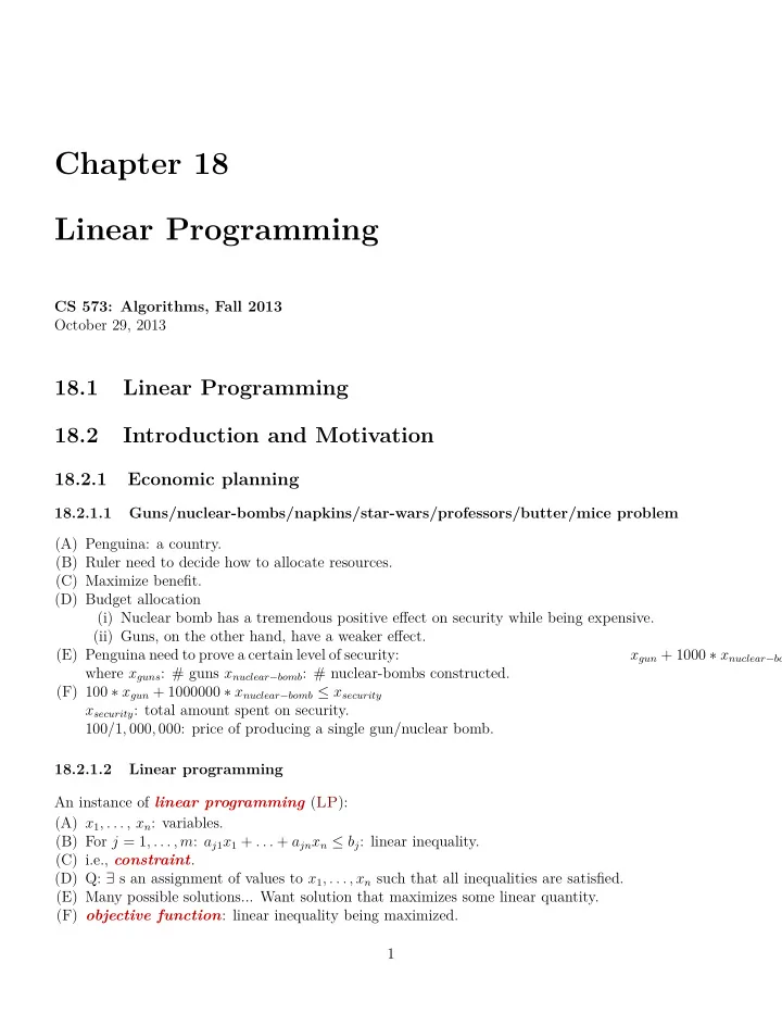
Chapter 18 Linear Programming CS 573: Algorithms, Fall 2013 October 29, 2013 18.1 Linear Programming 18.2 Introduction and Motivation 18.2.1 Economic planning 18.2.1.1 Guns/nuclear-bombs/napkins/star-wars/professors/butter/mice problem (A) Penguina: a country. (B) Ruler need to decide how to allocate resources. (C) Maximize benefit. (D) Budget allocation (i) Nuclear bomb has a tremendous positive effect on security while being expensive. (ii) Guns, on the other hand, have a weaker effect. (E) Penguina need to prove a certain level of security: x gun + 1000 ∗ x nuclear − bomb where x guns : # guns x nuclear − bomb : # nuclear-bombs constructed. (F) 100 ∗ x gun + 1000000 ∗ x nuclear − bomb ≤ x security x security : total amount spent on security. 100/1 , 000 , 000: price of producing a single gun/nuclear bomb. 18.2.1.2 Linear programming An instance of linear programming ( LP ): (A) x 1 , . . . , x n : variables. (B) For j = 1 , . . . , m : a j 1 x 1 + . . . + a jn x n ≤ b j : linear inequality. (C) i.e., constraint . (D) Q: ∃ s an assignment of values to x 1 , . . . , x n such that all inequalities are satisfied. (E) Many possible solutions... Want solution that maximizes some linear quantity. (F) objective function : linear inequality being maximized. 1

18.2.1.3 Linear programming – example a 11 x 1 + . . . + a 1 n x n ≤ b 1 a 21 x 1 + . . . + a 2 n x n ≤ b 2 . . . a m 1 x 1 + . . . + a mn x n ≤ b m max c 1 x 1 + . . . + c n x n . 18.2.1.4 History (A) 1939: L. V. Kantorovich noticed the importance of certain type of Linear Programming problems for resource allocation. (B) 1947: Dantzig invented the simplex method for solving LP problems for the US Air force planning problems. (C) 1947: T. C. Koopmans showed LP provide the right model for the analysis of classical economic theories. (D) 1975: Koopmans and Kantorovich got the Nobel prize of economics. (E) Kantorovich the only the Russian economist that got the Nobel prize 18.2.1.5 Network flow via linear programming Input: G = ( V , E ) with source s and sink t , and capacities c ( · ) on the edges. Compute max flow in G . ∀ ( u → v ) ∈ E 0 ≤ x u → v x u → v ≤ c ( u → v ) ∑ ∑ ∀ v ∈ V \ { s , t } x u → v − x v → w ≤ 0 ( u → v ) ∈ E ( v → w ) ∈ E ∑ ∑ x u → v − x v → w ≥ 0 ( u → v ) ∈ E ( v → w ) ∈ E maximizing ( s → u ) ∈ E x s → u ∑ 18.3 The Simplex Algorithm 18.4 The Simplex Algorithm 18.4.1 Linear program where all the variables are positive 18.4.1.1 Rewriting an LP n ∑ max c j x j j =1 n ∑ subject to a ij x j ≤ b i for i = 1 , 2 , . . . , m (A) Rewrite: so every variable is non-negative. j =1 (B) Replace variable x i by x ′ i and x ′′ i , where new constraints are: x i = x ′ i − x ′′ i , x ′ i ≥ 0 and x ′′ i ≥ 0. 2

(C) Example: The (silly) LP 2 x + y ≥ 5 rewritten: 2 x ′ − 2 x ′′ + y ′ − y ′′ ≥ 5, x ′ ≥ 0, y ′ ≥ 0, x ′′ ≥ 0, and y ′′ ≥ 0. 18.4.1.2 Rewriting an LP into standard form Lemma 18.4.1. Given an instance I of LP , one can rewrite it into an equivalent LP , such that all the variables must be non-negative. This takes linear time in the size of I . An LP where all variables must be non-negative is in standard form 18.4.2 Standard form 18.4.2.1 Standard form of LP A linear program in standard form. n ∑ max c j x j j =1 n ∑ subject to a ij x j ≤ b i for i = 1 , 2 , . . . , m j =1 x j ≥ 0 for j = 1 , . . . , n. 18.4.3 Standard form of LP 18.4.3.1 Because everything is clearer when you use matrices. Not.   a 11 a 12 . . . a 1( n − 1) a 1 n c, b and A : prespec- a 21 a 22 . . . a 2( n − 1) a 2 n     ified. x is vector of . .   . . A = ,  . . . . . . . . . . .  unknowns.     a ( m − 1)1 a ( m − 1)2 . . . a ( m − 1)( n − 1) a ( m − 1) n Solve LP for x .     a m 1 a m 2 . . . a m ( n − 1) a mn LP in standard form.   x 1 (Matrix notation.)     c 1 b 1 x 2     . . . c T x   max . . . c =   , b =     , x = . . . .             s.t. Ax ≤ b. c n b m x n − 1     x n x ≥ 0 . 18.4.4 Slack Form 18.4.4.1 Slack Form (A) Next rewrite LP into slack form . c T x max (B) Every inequality becomes equality. subject to Ax = b. (C) All variables must be positive. x ≥ 0 . (D) See resulting form on the right. 3

(A) New slack variables . Rewrite inequality: ∑ n i =1 a i x i ≤ b . As: n ∑ x n +1 = b − a i x i i =1 x n +1 ≥ 0 . (B) Value of slack variable x n +1 encodes how far is the original inequality for holding with equality. 18.4.4.2 Slack form... (A) LP now made of equalities of the form: x n +1 = b − ∑ n i =1 a i x i (B) Variables on left: basic variables . (C) Variables on right: nonbasic variables . (D) LP in this form is in slack form . Linear program in slack form. ∑ max z = v + c j x j , j ∈ N ∑ s.t. x i = b i − a ij x j for i ∈ B, j ∈ N x i ≥ 0 , ∀ i = 1 , . . . , n + m. 18.4.5 Slack form formally 18.4.5.1 Because everything is clearer when you use tuples. Not. B - Set of indices of basic variables N - Set of indices of nonbasic variables n = | N | - number of original variables b, c - two vectors of constants The slack form is defined by a tuple ( N, B, A, b, c, v ). m = | B | - number of basic variables (i.e., number of inequalities) A = { a ij } - The matrix of coefficients N ∪ B = { 1 , . . . , n + m } v - objective function constant. 18.4.6 Slack form formally 18.4.6.1 Final form ∑ Max z = v + c j x j , j ∈ N ∑ s.t. x i = b i − a ij x j for i ∈ B, j ∈ N x i ≥ 0 , ∀ i = 1 , . . . , n + m. 18.4.6.2 Example Consider the following LP which is in slack form. 4

z = 29 − 1 9 x 3 − 1 9 x 5 − 2 max 9 x 6 x 1 = 8 + 1 6 x 3 + 1 6 x 5 − 1 3 x 6 x 2 = 4 − 8 3 x 3 − 2 3 x 5 + 1 3 x 6 x 4 = 18 − 1 2 x 3 + 1 2 x 5 18.4.6.3 Example ...translated into tuple form ( N, B, A, b, c, v ). B = { 1 , 2 , 4 } , N = { 3 , 5 , 6 }     a 13 a 15 a 16 − 1 / 6 − 1 / 6 1 / 3 A = a 23 a 25 a 26  = 8 / 3 2 / 3 − 1 / 3        a 43 a 45 a 46 1 / 2 − 1 / 2 0         b 1 8 c 3 − 1 / 9 b = b 2 c = c 5 − 1 / 9  = 4  =               b 4 c 6 − 2 / 9 18 v = 29 . Note that indices depend on the sets N and B , and also that the entries in A are negation of what they appear in the slack form. 18.4.6.4 Another example... max 5 x 1 + 4 x 2 + 3 x 3 s.t. 2 x 1 + 3 x 2 + x 3 ≤ 5 4 x 1 + x 2 + 2 x 3 ≤ 11 3 x 1 + 4 x 2 + 2 x 3 ≤ 8 x 1 , x 2 , x 3 ≥ 0 Transform into slack form... max z = 5 x 1 + 4 x 2 + 3 x 3 s.t. w 1 = 5 − 2 x 1 − 3 x 2 − x 3 w 2 = 11 − 4 x 1 − x 2 − 2 x 3 w 3 = 8 − 3 x 1 − 4 x 2 − 2 x 3 x 1 , x 2 , x 3 , w 1 , w 2 , w 3 ≥ 0 5

18.4.7 The Simplex algorithm by example 18.4.7.1 The Simplex algorithm by example max 5 x 1 + 4 x 2 + 3 x 3 Next, we introduce slack variables, for exam- s.t. 2 x 1 + 3 x 2 + x 3 ≤ 5 ple, rewriting 2 x 1 + 3 x 2 + x 3 ≤ 5 as the con- 4 x 1 + x 2 + 2 x 3 ≤ 11 straints: w 1 ≥ 0 and w 1 = 5 − 2 x 1 − 3 x 2 − x 3 . The resulting LP in slack form is 3 x 1 + 4 x 2 + 2 x 3 ≤ 8 x 1 , x 2 , x 3 ≥ 0 max z = 5 x 1 + 4 x 2 + 3 x 3 s.t. w 1 = 5 − 2 x 1 − 3 x 2 − x 3 ⇒ w 2 = 11 − 4 x 1 − x 2 − 2 x 3 w 3 = 8 − 3 x 1 − 4 x 2 − 2 x 3 x 1 , x 2 , x 3 , w 1 , w 2 , w 3 ≥ 0 18.4.7.2 Example continued... (A) w 1 , w 2 , w 3 : slack variables. (Also currently max z = 5 x 1 + 4 x 2 + 3 x 3 basic variables). s.t. w 1 = 5 − 2 x 1 − 3 x 2 − x 3 (B) Consider the slack representation trivial so- lution... w 2 = 11 − 4 x 1 − x 2 − 2 x 3 all non-basic variables assigned zero: w 3 = 8 − 3 x 1 − 4 x 2 − 2 x 3 x 1 = x 2 = x 3 = 0. x 1 , x 2 , x 3 , w 1 , w 2 , w 3 ≥ 0 (A) = ⇒ w 1 = 5, w 2 = 11 and w 3 = 8. (B) Feasible! (C) Objection function value: z = 0. (D) Further improve t value of objective function (i.e., z ). While keeping feasibility. 18.4.7.3 Example continued... max z = 5 x 1 + 4 x 2 + 3 x 3 (A) x 1 = x 2 = x 3 = 0 = ⇒ w 1 = 5, w 2 = 11 s.t. w 1 = 5 − 2 x 1 − 3 x 2 − x 3 and w 3 = 8. (B) All w i positive – change x i a bit does not w 2 = 11 − 4 x 1 − x 2 − 2 x 3 change feasibility. w 3 = 8 − 3 x 1 − 4 x 2 − 2 x 3 x 1 , x 2 , x 3 , w 1 , w 2 , w 3 ≥ 0 (A) z = 5 x 1 + 4 x 2 + 3 x 3 : want to increase values of x 1 s... since z increases (since 5 > 0). (B) How much to increase x 1 ??? (C) Careful! Might break feasibility. (D) Increase x 1 as much as possible without breaking feasibility! 6