Optimization Theory and n n n 1 minimize - - PowerPoint PPT Presentation

SLIDE 1

OptimizationTheoryand DualityforSVMs

Outline:

• Toolsfordesigninglearning(training)algorithms.
• Howtomaketheoptimizationproblemmoretractable?
• Adualrepresentationoftheoptimalhyperplaneintermsofthe

trainingexamples.

• Whatinsightdowegainfromthedualrepresentation?
• Whatarethepropertiesofthedualoptimizationproblem?

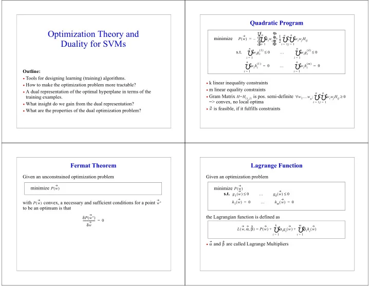
QuadraticProgram

• klinearinequalityconstraints
• mlinearequalityconstraints
• GramMatrix

ispos.semi-definite =>convex,nolocaloptima

• isfeasible,ifitfulfillsconstraints

minimize s.t.

P w ( ) kiwi

i 1 = n

• –

1 2

• wiwjHij

j 1 = n

• i

1 = n

• +

= wigi

1 ( ) i 1 = n

• ≤

… wigi

k ( ) i 1 = n

• ≤

wihi

1 ( ) i 1 = n

• =

… wihi

m ( ) i 1 = n

• =

H H i j

, ( )

= w1…wn wiwjHij

j 1 = n

• i

1 = n

• ;

∀ ≥ w

FermatTheorem

Givenanunconstrainedoptimizationproblem with convex,anecessaryandsufficientconditionsforapoint

• tobeanoptimumisthat

minimize

• P w

( ) P w ( ) w° δP w° ( ) δw

• =

LagrangeFunction

Givenanoptimizationproblem theLagrangianfunctionisdefinedas

• and arecalledLagrangeMultipliers

minimize s.t.

• P w

( ) g1 w ( ) ≤ … gk w ( ) ≤ h1 w ( ) = … hm w ( ) =

• L w α β

, , ( ) P w ( ) αigi w ( )

i 1 = k

• βihi w

( )

i 1 = m

• +

+ = α β

SLIDE 2

LagrangeTheorem

Givenanoptimizationproblem with convexandallhaffine(w*x+b),necessaryandsufficient conditionsforapoint tobeanoptimumaretheexistenceof such that => minimize s.t.

P w ( ) h1 w ( ) = … hm w ( ) = P w ( ) w° β° δL w° β° , ( ) δw

• =

δL w° β° , ( ) δβ

• =

L w β , ( ) P w ( ) βihi w ( )

i 1 = m

• +

= L w° β , ( ) L w° β° , ( ) L w β° , ( ) ≤ ≤

Karush-Kuhn-TuckerTheorem

Givenanoptimizationproblem with convexandallgandhaffine,necessaryandsufficient conditionsforapoint tobeanoptimumaretheexistenceof and

• suchthat

SufficientforconvexQP: minimize s.t.

• P w

( ) g1 w ( ) ≤ … gk w ( ) ≤ h1 w ( ) = … hm w ( ) = P w ( ) w° α° β° δL w° α° β° , , ( ) δw

• =

δL w° α° β° , , ( ) δβ

• =

αi°gi w° ( ) 0 i , 1 … k , , = = gi w° ( ) 0 i , ≤ 1 … k , , = αi° 0 i , ≥ 1 … k , , = max

α 0 β , ≥

min

wL w α β

, , ( )

DualOptimizationProblem

Lemma:Thesolution canalwaysbewrittenasalinearcombination

• fthetrainingdata.

==>Lagrangemultipliers ==>positivesemi-definitequadraticprogram PrimalOP:minimize ,with

P w b , ( ) 1 2

• w w

⋅ = i yi w xi ⋅ b + [ ] 1 ≥ ∀ w° w° αiyixi

i 1 = n

• =

αi ≥

DualOP:maximize s.t.

D α ( ) αi

i 1 = n

• 1

2

• αiαjyiyj xi xj

⋅ ( )

j 1 = n

• i

1 = n

• –

= αiyi

i 1 = n

• =

and αi ≤

Primal<=>Dual

Theorem:TheprimalOPandthedualOPhavethesamesolution. Giventhesolution

• fthedualOP,

isthesolutionoftheprimalOP. Theorem:Foranyfeasiblepoints . =>twoalternativewaystorepresentthelearningresult

• weightvectorandthreshold
• vectorof“ influences”
• αi°

w° αi °yixi

i 1 = n

• =

b° 1 2

• w0 x

pos

⋅ w0 x

neg

⋅ + ( ) = P w b , ( ) D α ( ) ≥ w b ,

• α1 … αn

, ,

SLIDE 3

PropertiesoftheDualOP

• singlesolution(i.e.

isunique)

• onefactor

foreachtrainingexample

• describesthe“ influence” oftraining

examplesiontheresult

• <=>trainingexampleisasupport

vector

• else
• dependsexclusivelyoninnerproduct

betweentrainingexamples DualOP:maximize s.t.

D α ( ) αi

i 1 = n

• 1

2

• αiαjyiyj xi xj

⋅ ( )

j 1 = n

• i

1 = n

• –

= αiyi

i 1 = n

• =

and αi ≤ w b ,

• δ

αi αi > αi =

PropertiesoftheSoft-MarginDualOP

• (mostly)singlesolution(i.e.

isalmostalwaysunique)

• onefactor

foreachtrainingexample

• “ influence” ofsingletraining

examplelimitedbyC

• <=>SVwith
• <=>SVwith
• else
• basedexclusivelyoninnerproduct

betweentrainingexamples DualOP:maximize s.t.

D α ( ) αi

i 1 = n

• 1

2

• αiαjyiyj xi xj

⋅ ( )

j 1 = n

• i

1 = n

• –

= αiyi

i 1 = n

• =

and αi C ≤ ≤ w b ,

• ξi

ξj αi αi C < < ξi = αi C = ξi > αi =