
SLIDE 1
Unit 1A 1
Chang, Huang, Li, Lin, Liu
Unit 1A: Computational Complexity
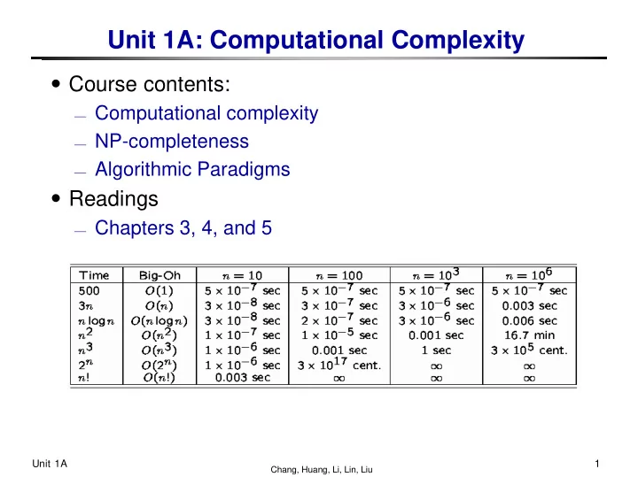
․Course contents:
⎯ Computational complexity ⎯ NP-completeness ⎯ Algorithmic Paradigms
․Readings
⎯ Chapters 3, 4, and 5
Optimization Problems Problem: a general class, e.g., the - - PowerPoint PPT Presentation
Unit 1A: Computational Complexity Course contents: Computational complexity NP-completeness Algorithmic Paradigms Readings Chapters 3, 4, and 5 Unit 1A 1 Chang, Huang, Li, Lin, Liu O : Upper Bounding Function Def: f (
Unit 1A 1
Chang, Huang, Li, Lin, Liu
⎯ Computational complexity ⎯ NP-completeness ⎯ Algorithmic Paradigms
⎯ Chapters 3, 4, and 5
Unit 1A 2
Chang, Huang, Li, Lin, Liu
⎯ Examples: 2n2 + 3n = O(n2), 2n2 = O(n3), 3n lg n = O(n2)
Unit 1A 3
Chang, Huang, Li, Lin, Liu
⎯ f(n) = O(g(n)) iff limn → ∞
Unit 1A 4
Chang, Huang, Li, Lin, Liu
⎯ sort n words of bounded length ⇒ n ⎯ the input is the integer n ⇒ lg n ⎯ the input is the graph G(V, E) ⇒ |V| and |E|
Unit 1A 5
Chang, Huang, Li, Lin, Liu
⎯ 999: constant ⎯ lg n: logarithmic ⎯
⎯ n: linear ⎯ n lg n: loglinear ⎯ n2: quadratic ⎯ n3: cubic
⎯ 2n, 3n: exponential ⎯ n!: factorial
Unit 1A 6
Chang, Huang, Li, Lin, Liu
Unit 1A 7
Chang, Huang, Li, Lin, Liu
⎯ MST: Given a graph G=(V, E), find the cost of a minimum
⎯ F is the set of feasible solutions, and ⎯ c is a cost function, assigning a cost value to each feasible
⎯ The solution of the optimization problem is the feasible solution
Unit 1A 8
Chang, Huang, Li, Lin, Liu
Unit 1A 9
Chang, Huang, Li, Lin, Liu
⎯ MST: Given a graph G=(V, E) and a bound K, is there a
⎯ TSP: Given a set of cities, distance between each pair of cities,
⎯ The set of of instances for which the answer is “yes” is given
⎯ A subtask of a decision problem is solution checking: given f ∈
Unit 1A 10
Chang, Huang, Li, Lin, Liu
⎯ Instance: A combinational circuit C composed of AND, OR,
⎯ Question: Is there an assignment of Boolean values to the
⎯ Circuit (a) is satisfiable since <x1, x2, x3> = <1, 1, 0> makes the
Unit 1A 11
Chang, Huang, Li, Lin, Liu
⎯ Input size: size of encoded “binary” strings. ⎯ Edmonds: Problems in P are considered tractable.
⎯ Deterministic means that each step in a computation is
⎯ A Turing machine is a mathematical model of a
Unit 1A 12
Chang, Huang, Li, Lin, Liu
⎯ Nondeterministic: the machine makes a guess, e.g., the right
⎯ NP: class of problems that can be solved in polynomial time on
⎯ Need to check a solution in polynomial time.
Guess a tour. Check if the tour visits every city exactly once. Check if the tour returns to the start. Check if total distance ≤ B.
⎯ All can be done in O(n) time, so TSP ∈ NP.
Unit 1A 13
Chang, Huang, Li, Lin, Liu
⎯ Developed by S. Cook and R. Karp in early 1970. ⎯ All problems in NPC have the same degree of difficulty: Any
Unit 1A 14
Chang, Huang, Li, Lin, Liu
⎯ f reduces input for L1 into an input for L2 s.t. the reduced input is
L1 ≤ P L2 if ∃ polynomial-time computable function f: {0, 1}*→
L2 is at least as hard as L1.
Unit 1A 15
Chang, Huang, Li, Lin, Liu
⎯ ∃ polynomial-time algorithm for L2 ⇒ ∃ polynomial-time
⎯
Unit 1A 16
Chang, Huang, Li, Lin, Liu
⎯
⎯
1.
2.
Unit 1A 17
Chang, Huang, Li, Lin, Liu
Unit 1A 18
Chang, Huang, Li, Lin, Liu
— x ∈ HC ⇒ f(x) ∈ TSP.
— Suppose the HC is h = <v1, v2, …, vn, v1>. Then, h is also a
— The distance of the tour h is n = B since there are n
— Thus, f(x) ∈ TSP (f(x) has a TSP tour with distance ≤ B).
Unit 1A 19
Chang, Huang, Li, Lin, Liu
— f(x) ∈ TSP ⇒ x ∈ HC.
— Suppose there is a TSP tour with distance ≤ n = B. Let it be
— Since distance of the tour ≤ n and there are n edges in the
— Thus, <v1, v2, …, vn, v1> is a Hamiltonian cycle (x ∈ HC).
Unit 1A 20
Chang, Huang, Li, Lin, Liu
⎯
⎯
⎯ If L ∈ P, then there exists a polynomial-time algorithm for every
⎯ If L ∉ P, then there exists no polynomial-time algorithm for any L'
Unit 1A 21
Chang, Huang, Li, Lin, Liu
1.
2.
3.
4.
5.
Unit 1A 22
Chang, Huang, Li, Lin, Liu
⎯ Guarantee to be a fixed percentage away from the optimum. ⎯ E.g., MST for the minimum Steiner tree problem.
⎯ Has the form of a polynomial function for the complexity, but is
⎯ E.g., O(nW) for the 0-1 knapsack problem.
⎯ Work on some subset of the original problem. ⎯ E.g., the longest path problem in directed acyclic graphs.
⎯ Is feasible only when the problem size is small.
⎯ Simulated annealing (hill climbing), genetic algorithms, etc.
Unit 1A 23
Chang, Huang, Li, Lin, Liu
⎯ The spanning tree algorithm can be an approximation for the Steiner
Steiner points
Unit 1A 24
Chang, Huang, Li, Lin, Liu
Unit 1A 25
Chang, Huang, Li, Lin, Liu
Unit 1A 26
Chang, Huang, Li, Lin, Liu
⎯ Partition a problem into independent subproblems, solve the
⎯ Inefficient if they solve the same subproblem more than once.
⎯ Applicable when the subproblems are not independent. ⎯ DP solves each subproblem just once.
Unit 1A 27
Chang, Huang, Li, Lin, Liu
S = (1, 4, 2, 1, 2, 3, 5)
Unit 1A 28
Chang, Huang, Li, Lin, Liu
S = (1, 4, 2, 1, 2, 3, 5)
⎯ FFD(Π) ≤ 11OPT(Π)/9 + 4)
Unit 1A 29
Chang, Huang, Li, Lin, Liu
Unit 1A 30
Chang, Huang, Li, Lin, Liu
⎯ ACM/IEEE Design Automation Conference (DAC) ⎯ IEEE/ACM Int'l Conference on Computer-Aided Design (ICCAD) ⎯ IEEE Int’l Test Conference (ITC) ⎯ ACM Int'l Symposium on Physical Design (ISPD) ⎯ ACM/IEEE Asia and South Pacific Design Automation Conf. (ASP-DAC) ⎯ ACM/IEEE Design, Automation, and Test in Europe (DATE) ⎯ IEEE Int'l Conference on Computer Design (ICCD) ⎯ IEEE Custom Integrated Circuits Conference (CICC) ⎯ IEEE Int'l Symposium on Circuits and Systems (ISCAS) ⎯ Others: VLSI Design/CAD Symposium/Taiwan
⎯ IEEE Transactions on Computer-Aided Design (TCAD) ⎯ ACM Transactions on Design Automation of Electronic Systems
⎯ IEEE Transactions on VLSI Systems (TVLSI) ⎯ IEEE Transactions on Computers (TC) ⎯ IEE Proceedings – Circuits, Devices and Systems ⎯ IEE Proceedings – Digital Systems ⎯ INTEGRATION: The VLSI Journal