
SLIDE 1
ON NETWORKS OF INTERCONNECTED SYSTEMS
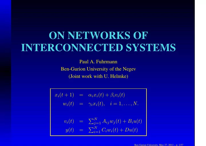
Paul A. Fuhrmann Ben-Gurion University of the Negev (Joint work with U. Helmke) xi(t + 1) = αixi(t) + βivi(t) wi(t) = γixi(t), i = 1, . . . , N. vi(t) = N
j=1 Aijwj(t) + Biu(t)
y(t) = N
i=1 Ciwi(t) + Du(t)
Ben Gurion University, May 27, 2012 – p. 1/37