On entropic cost optimal transport cost Soumik Pal University of - PowerPoint PPT Presentation

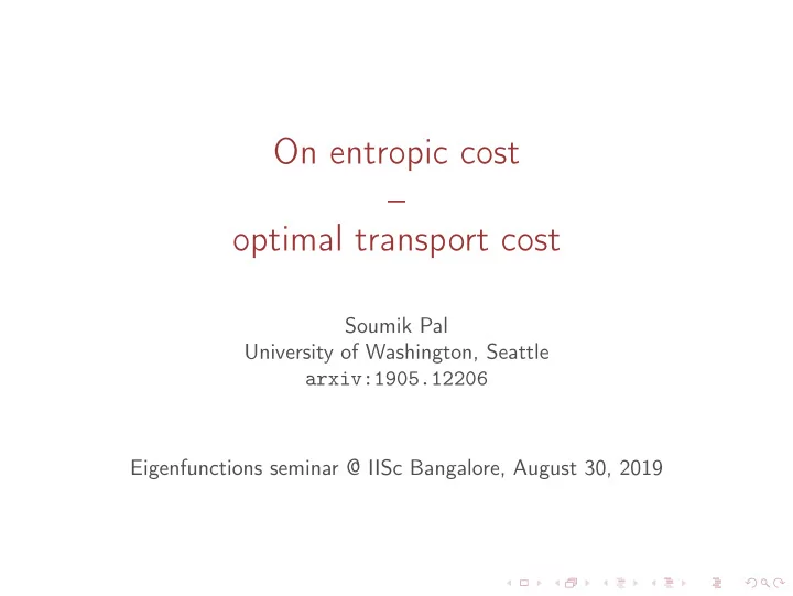
On entropic cost – optimal transport cost Soumik Pal University of Washington, Seattle arxiv:1905.12206 Eigenfunctions seminar @ IISc Bangalore, August 30, 2019

MK OT and entropic relaxation ρ 0 , ρ 1 - probability densities on X = R d = Y . c ( x , y ) = g ( x − y ) , strictly convex, g ≥ 0, g ( z ) = 0 iff z = 0. Π( ρ 0 , ρ 1 ) - set of couplings. Probabilities on X × Y . Monge-Kantorovich (MK) OT problem: � W g ( ρ 0 , ρ 1 ) := inf ν ∈ Π ν ( g ( x − y )) = inf g ( x − y ) d ν. ν ∈ Π Entropic relaxation (Cuturi, Peyré). For h > 0, � K ′ h := inf ν ∈ Π [ ν ( g ( x − y )) + h Ent ( ν )] , Ent ( ν ) = ν ( x ) log ν ( x ) dx Fast algorithms for h > 0. Want h → 0.

Entropic cost An equivalent form of entropic relaxation. Define “transition kernel”: � � p h ( x , y ) = 1 − 1 exp hg ( x − y ) , Λ h and joint distribution µ h ( x , y ) = ρ 0 ( x ) p h ( x , y ) . Relative entropy: � d ν � � H ( ν | µ ) = log d ν. d µ Define entropic cost K h = couplings ( ρ 0 ,ρ 1 ) H ( ν | µ h ) . inf K h = K ′ h / h − Ent ( ρ 0 ) + log Λ h

Example: quadratic Wasserstein 2 � x − y � 2 . Consider g ( x − y ) = 1 p h ( x , y ) - transition of Brownian motion. h = temperature. � � − 1 p h ( x , y ) = ( 2 π h ) − d / 2 exp 2 h � x − y � 2 . In general, there need not be a stochastic process for p h ( x , y ) . Theorem (Y. Brenier ’87) There exists unique convex φ such that T ( x ) = ∇ φ ( x ) solves both Monge and Kantorovich OT problems for ( ρ 0 , ρ 1 ) .

Schrödinger’s problem Brownian motion X - temperature h ≈ 0 “Condition” X 0 ∼ ρ 0 , X 1 ∼ ρ 1 . Exponentially rare. On this rare event what do particles do? Schrödinger ’31, Föllmer ’88, Léonard ’12. Particle initially at x moves close to ∇ φ ( x ) (Brenier map). In fact, lim h → 0 hK h = 1 2 W 2 2 ( ρ 0 , ρ 1 ) . True in general. For any g ( x − y ) : h → 0 hK h = W g ( ρ 0 , ρ 1 ) . lim Rate of convergence?

Pointwise convergence Theorem (P. ’19) ρ 0 , ρ 1 compactly supported and continuous (+ smoothness etc.). Kantorovich potential uniformly convex. � � K h − 1 = 1 2 h W 2 lim 2 ( ρ 0 , ρ 1 ) 2 ( Ent ( ρ 1 ) − Ent ( ρ 0 )) . h → 0 + Complementary results known for gamma convergence. Pointwise convergence left open. Adams, Dirr, Peletier, Zimmer ’11 (1-d), Duong, Laschos, Renger ’13, Erbar, Maas, Renger ’15 (multidimension, Fokker-Planck).

Divergence To state the result for a general g , need a new concept. For a convex function φ , Bregman divergence: D [ y | z ] = φ ( y ) − φ ( z ) − ( y − z ) · ∇ φ ( z ) ≥ 0 . If x ∗ = ∇ φ ( x ) , D [ y | x ∗ ] = 1 2 � y − x � 2 − φ c ( x ) − φ ∗ c ( y ) , where φ c , φ ∗ c are c-concave functions: φ c ( x ) = 1 c ( y ) = 1 2 � x � 2 − φ ( x ) , 2 � y � 2 − φ ∗ ( y ) . φ ∗ y ≈ x ∗ , D [ y | x ∗ ] ≈ ( y − x ∗ ) T A ( x ∗ )( y − x ∗ ) , A ( z ) = ∇ 2 φ ∗ ( z ) .

Divergence Generalize to cost g . Monge solution given by (Gangbo - McCann) x ∗ = x − ( ∇ g ) − 1 ◦ ∇ ψ, for some c -concave function ψ . Dual c-concave function ψ ∗ . Divergence D [ y | x ∗ ] = g ( x − y ) − ψ ( x ) − ψ ∗ ( y ) ≥ 0 . y ≈ x ∗ , extract matrix A ( x ∗ ) from the Taylor series. Divergence/ A ( · ) measures sensitivity of Monge map. Related to cross-difference of Kim & McCann ’10, McCann ’12, Yang & Wong ’19.

Pointwise convergence Theorem (P. ’19) ρ 0 , ρ 1 compactly supported, continuous (+ smoothness etc.). A ( · ) “uniformly elliptic”. � � � K h − 1 = 1 ρ 1 ( y ) log det( A ( y )) dy − 1 2 log det ∇ 2 g ( 0 ) . lim h W g ( ρ 0 , ρ 1 ) 2 h → 0 + For g ( x − y ) = � x − y � 2 / 2, log det ∇ 2 g ( 0 ) = 0, for φ (Brenier) � � 1 ρ 1 ( y ) log det( A ( y )) dy = 1 ρ 1 ( y ) log det( ∇ 2 φ ∗ ( y )) dy , 2 2 which is 1 2 ( Ent ( ρ 1 ) − Ent ( ρ 0 )) by simple calculation a la McCann.

The Dirichlet transport

Dirichlet transport, P.-Wong ’16 ∆ n - unit simplex { ( p 1 , . . . , p n ) : p i > 0 , � i p i = 1 } . ∆ n is an abelian group. e = ( 1 / n , . . . , 1 / n ) If p , q ∈ ∆ n , then � p − 1 � p i q i 1 / p i ( p ⊙ q ) i = � n , i = � n . j = 1 p j q j j = 1 1 / p j K-L divergence or relative entropy as “distance”: n � H ( q | p ) = q i log( q i / p i ) . i = 1 Take X = Y = ∆ n . � � � n � n � � 1 q i − 1 log q i e | p − 1 ⊙ q c ( p , q ) = H = log ≥ 0 . n p i n p i i = 1 i = 1

Some economic motivation Market weights for n stocks: µ = ( µ 1 , . . . , µ n ) . µ i = Proportion of the total capital that belongs to i th stock. Investment portfolio: π = ( π 1 , . . . , π n ) ∈ ∆ n . Portfolio weights: π i = Proportion of the total value that belongs to i th stock . Markovian investments π = π ( µ ) : ∆ n → ∆ n . How to build robust portfolios that compare with an index, say, S&P 500? ONLY solutions given by the Dirichlet transport.

Exponentially concave functions ϕ : ∆ n → R ∪ {−∞} is exponentially concave if e ϕ is concave. x �→ 1 2 log x is e-concave, but not x �→ 2 log x . Examples: p , r ∈ ∆ n , 0 < λ < 1. � ϕ ( p ) = 1 log p i . n i �� � �� � ϕ ( p ) = 1 p λ ϕ ( p ) = log r i p i , λ log . i i i (Fernholz ’02, P. and Wong ’15). Analog of Brenier’s Theorem: If ( p , q = F ( p )) is the Monge solution, then p − 1 = � ∇ ϕ ( q ) , Kantorovich potential . Smooth, MTW Khan & Zhang ’19.

Back to the Dirichlet transport What is the corresponding probabilistic picture for the cost function � � e | p − 1 ⊙ q c ( p , q ) = H on the unit simplex ∆ n ? Symmetric Dirichlet distribution Dir ( λ ) : � n p λ/ n − 1 density ∝ . j j = 1 Probability distribution on the unit simplex. If U ∼ Dir ( · ) , � 1 � E ( U ) = e , Var ( U i ) = O . λ

Dirichlet transition Haar measure on (∆ n , ⊙ ) is Dir ( 0 ) , ν ( p ) = � n i = 1 p − 1 . i Consider transition probability: p ∈ ∆ n , U ∼ Dir ( λ ) , Q = p ⊙ U . f λ ( p , q ) = c ν ( q ) exp ( − λ c ( p , q )) , (P.-Wong ’18) . Temperature: h = 1 λ . Let p h ( p , q ) = f 1 / h ( p , q ) . As h → 0 + , p h → δ p . As h → ∞ , Q → Dir ( 0 ) , Haar measure.

Multiplicative Schrödinger problem Fix ρ 0 , ρ 1 . Let µ h ( p , q ) = ρ 0 ( p ) p h ( p , q ) . � Recall relative entropy: H ( ν | µ ) = log( d ν/ d µ ) d µ . Entropic cost K h = couplings ( ρ 0 ,ρ 1 ) H ( ν | µ h ) inf For ρ density on ∆ n , let Ent 0 ( ρ ) = H ( ρ | Dir ( 0 )) . Relative entropy w.r.t. Haar measure.

Pointwise convergence Theorem (P. ’19) ρ 0 , ρ 1 are compactly supported + exponentially concave potential is “uniformly convex”. � � 1 � � = 1 h − n lim K h − C ( ρ 0 , ρ 1 ) 2 ( Ent 0 ( ρ 1 ) − Ent 0 ( ρ 0 )) . 2 h → 0 + C ( ρ 0 , ρ 1 ) is the optimal cost of transport with cost c . Not a metric, but a divergence. Not symmetric in ( ρ 0 , ρ 1 ) . AFAIK, the only such example known. Related to Erbar ’14 (jump processes), and Maas ’11 (Markov chains).

Idea of the proof: approximate Schrödinger bridge

Idea of the proof: Brownian case Recall, want to condition Brownian motion to have marginals ρ 0 , ρ 1 . p h ( x , y ) Brownian transition density at time h . µ h ( x , y ) = ρ 0 ( x ) p h ( x , y ) , joint distribution . If I can “guess” this conditional distribution ν h , then K h = couplings ( ρ 0 ,ρ 1 ) H ( ν | µ h ) = H ( � inf µ h | µ h ) . Can approximately do so for small h by a Taylor expansion in h .

Idea of the proof: Brownian case It is known (Rüschendorf) that � µ h must be of the form � � − 1 µ h ( x , y ) = e a ( x )+ b ( y ) µ h ( x , y ) ∝ exp � hg ( x − y ) + a ( x ) + b ( y ) . φ - convex function from Brenier map. � � � � � x � 2 | y | 2 a ( x ) = 1 + h ζ h ( x ) , b ( y ) = 1 − φ ∗ ( y ) − φ ( x ) + h ξ h ( y ) , h 2 h 2 ζ h , ξ h are O ( 1 ) .

Idea of the proof Thus, up to lower order terms, � � − 1 hg ( x − y ) + 1 h φ c ( x ) + 1 h φ ∗ � µ h ( x , y ) ∝ ρ 0 ( x ) exp c ( y ) � � − 1 = ρ 0 ( x ) exp hD [ y | x ∗ ] . If y − x ∗ is large, it gets penalized exponentially. Hence � � − 1 2 h ( y − x ∗ ) T ∇ 2 φ ∗ ( x ∗ )( y − x ∗ ) µ h ( x , y ) ∝ ρ 0 ( x ) exp � Gaussian transition kernel with mean x ∗ and covariance � � − 1 . ∇ 2 φ ∗ ( x ∗ ) h

Idea of the proof For h ≈ 0, the Schrödinger bridge is approximately Gaussian. � � − 1 � � x ∗ , h ∇ 2 φ ∗ ( x ∗ ) Sample X ∼ ρ 0 , generate Y ∼ N . 1 ( 2 π h ) − d / 2 × µ h ( x , y ) ≈ ρ 0 ( x ) � � det( ∇ 2 φ ∗ ( x ∗ )) � � − 1 2 h ( y − x ∗ ) T ∇ 2 φ ∗ ( x ∗ )( y − x ∗ ) exp . Y is not exactly ρ 1 . Lower order corrections. Nevertheless, � µ h | µ h ) = 1 det ∇ 2 φ ∗ ( x ∗ ) ρ 0 ( x ) dx = 1 H ( � 2 ( Ent ( ρ 1 ) − Ent ( ρ 0 )) . 2