Off-critical SLEs: Massive SLE(4) with M. Bauer, Saclay. A sample - - PowerPoint PPT Presentation

Off-critical SLEs: Massive SLE(4)

with M. Bauer, Saclay.

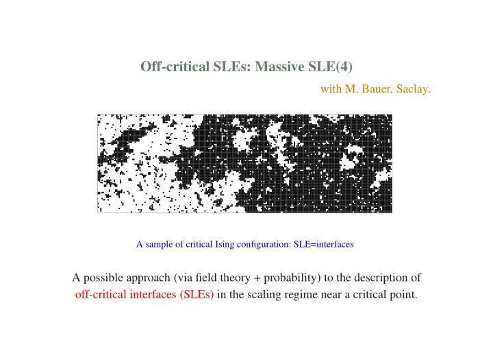
A sample of critical Ising configuration: SLE=interfaces

A possible approach (via field theory + probability) to the description of

• ff-critical interfaces (SLEs) in the scaling regime near a critical point.

Many examples: – Ising model at T → Tc; – Percolation at p → pc; – LERW at x → xc; – SAW at different fugacity; – etc... Break conformal invariance Loop Erased Random Walks: Weight: wγ = ∑r→γ x|r| At criticality xc

Plan:

• Toy model: random walks
• SAW as an example
• Drift, partition function and field theory
• Massive SLE(4)
• Massive LERW

A toy model: random walks

• Let XN = a∑N

j=1 ε j be a (biaised) random walks of step a,

with ε j = ± with proba p, 1− p. Set Xt = a(N+ −N−) and t = a2N = a2(N+ +N−). The scaling limit is for N → ∞, a → 0 at t fixed: At ”criticality” pc = 1/2, Xt =Brownian motion: (dXt)2 = dt.

• ”Near criticality” p → 1/2 as a → 0?

The ratio of proba of a walk at p and pc is (2p)N+(2(1− p))N−, so: Ep[···] = Ep=1/2[M···] with M ≡ eS = (2p)N+(2(1− p))N− To get a finite weight M, we need p ≃ (1+aµ)/2 as a → 0 (scaling limit). The ’action’ is then St = µXt −µ2t/2 and in the continuum: Eµ[···] = EBr[Mt ···] with Mt ≡ eSt = eµXt−µ2t/2 (a martingale) W.r.t. Eµ, Xt now has a drift: dXt = dBt +µdt.

• A martingale for some stochastic process is a time dependent random

variable, say t → Mt, such that its expectation conditioned on the process up to time s is Ms, i.e. statistically conserved quantity.

• Going off-criticality amounts to weight by a martingale (which depends
• n the perturbation). It modifies (adds a drift to) the stochastic equation.

This is the approach we (try to) adapt to off-critical SLEs.......

• Grisanov theorem:

If Mt martingale for Brownian motion Xt: M−1

t

dMt = F

tdXt,

then w.r.t. to ˆ E[···] = EBr[Mt ···], Xt satisfies dXt = d ˆ Bt +F

tdt with ˆ

Bt a ˆ E-Brownian motion. In physics, this is known as the M.S.R. path integral representation.

• Other works on off-critical SLEs: Nolin-Werner, Makarov-Smirnov, ...

SAW as an example

SAW= self-avoiding walk Weight: wγ = x|γ| with |γ| = nbr. steps. Proba: wγ/ZD with ZD = ∑γ wγ the partition function. At criticality x = xc, conjecturally SAW=SLE(8/3) in the continuum, a → 0.

• How to take the scaling limit?

ZD/Zcrit.

D

= Zcrit.

D −1∑ γ

x|γ| = Zcrit.

D −1∑ γ

x|γ|

c (x/xc)|γ| = Ecrit.[(x/xc)|γ|]

At criticality, |γ| is related to the macroscopic size via the fractal dimension: |γ| ≃ [ℓ(γ)/a]dκ. The scaling limit is x−xc

xc

≃ −adκµ and: ZD/Zcrit.

D

= Ecrit.[e−µLD(γ)] , LD(γ) ≃ adκ|γ| ≡ ′natural parametrisation′

• Off-critical weight, off-critical drift and partition function.

(For SAW) the off-critical weighting is by the natural parametrization: Eµ[O] = Z−1

D Ecrit.[e−µLD(γ)O] with ZD = Ecrit.[e−µLD(γ)].

If the observable O only depends on the curve up to time t (Ft-measurable): Eµ[O] = Ecrit.[Mt O] with Mt = Z−1

D Ecrit.[e−µLD(γ)|Ft]

Girsanov theorem tells that the off-critical drift is M−1

t

dMt. Since LD(γ) counts the number of steps, we expect an additivity pro- perty: LD(γ[0,s]) = LD(γ[0,t])+LD\γ[0,t](γ[t,s]) For the off-critical weighting martingale = ⇒ Mt = e−µLD(γ[0,t]) ZD\γ[0,t]

ZD

Ie.→ ”surface energy” + ”ratio of partition function”.

Off-critical SLE and field theory

Loewner equation: dgt(z) dt = 2 gt(z)−ξt

ξt: driving source.

• At criticality, ξt is a 1D Brownian motion, E[ξ2

t ] = κt.

• Off-criticality, ξt not a Brownian motion (it depends on the perturbation):

— short distance: by scaling we expect: λ−1ξλ2t → √κBt as λ → 0. — decomposition: from above, we expect: dξt = √κdBt +F

tdt

F

t off-critical drift term (perturbation dependent).

— But off-critical measure can be singular w.r.t. critical one (cf percolation [Nolin-Werner] or infinite domain).

• From field theory, the off-critical drift reads

. F

t = M−1 t

dMt = κ∂ξt log(eEt(γ[0,t]) Zt). The off-critical weighting martingale Mt = eEt Zt with Zt = Zoff−crit.

t

/Zcrit.

t

, the ratio of the partition functions in the domain cut along the curve.

• Previous discussion follows (naively) from basic stat. mech. principles.

(because the measure on curves induced by the Boltzmann weights is the ratio of partition functions).

• The measure on curves is induced (via the Loewner equation) from that
• n the driving source ξt solution of the SDE: dξt = √κdBt +F

tdt.

Massive SLE(4)

To appear...

SLE(4) in a perturbed environment.

Massive bosonic free field S =

Z d2x

8π [(∂X)2 +m2(x)X2] with Dirichlet boundary conditions.

• SLE(4) = discontinuity curve of a massless boson (Sheffield-Schramm).
• At criticality, Gaussian free field (in upper half plane H):

X(z)H = √ 2 Im(logz) , X(z)X(w)conn.

H

= G0(z,w) = −log|z−w z− ¯ w|2 Perturbing (composite) operator: X2(z) = limw→z X(z)X(w)+log|z−w|2.

• Off-critical drift F

t = 4∂ξ logZ[m] t

with Z[m]

t

= e−

R d2x

8π m2(x)X2(x)Ht.

Ht = the cutted upper half plane.

• First order computation.

X2 is not a scalar but X2(z)Ht is a (local) martingale: X2(z)Ht = ϕt(z)2 +logρt(z), ϕt(z) = √ 2 Im(loggt(z)), ρt(z) = conf. radius To 1rst order, Z[m]

t

= 1−

R d2x

8π m2(x)X2(z)Ht +···.

As a CFT correlation, ϕt(z) is a martingale: dϕt(z) = θt(z)dBt. To 1rst order, the drift is: F

t = −

R d2x

4π m2(x) θt(x) ϕt(x)+···.

• All order computation.

Computable since the theory is Gaussian (only connected diagrams contribute), and to all orders: F

t = −

Z d2x

4π m2(x) θt(x) Φ[m]

t

(x) = −

Z d2x

4π m2(x) Θ[m]

t (x) ϕt(x)

with (−∆+m2)Φ[m]

t

= 0 in Ht with Dirichlet b.c.

• Massive X(x)Ht= (conditioned) proba for γ to be on the right of x.

It should be/It is a (massive) martingale with this drift.

This follows from Hadamard formula.

This is the way Makarov-Smirnov computed the drift.

• Perfect matching (should be true from basic stat. mech.):

E[m][ ···(any X correlation)···Ht ] = ···(any X correlation)···H → Reorganisation of the statistical sum: – first sum over fields at fixed interfaces – then on possible interfaces shapes.

• The curve γ is (a.s.) the discontinuity curve.
• Massive harmonic navigator (with killing)

Massive LERW

LERW=random walk with loop erased. Weight: wγ = ∑r→γ x|r| At criticality xc SLE(2) = [c=-2] = symplectic fermions.

• Scaling limit x−xc

xc

= −a2µ and the partition function ZD = ∑r x|r|: ZD = EBr.[e−µτD] = EBr.[exp(−

Z

d2x µ(x) ℓD(x))] Brownian local time ℓD(x) is conformal of dimension zero.

• Fugacity perturbation is the massive perturbation:

S =

Z d2x

8π [(∂χ+)(∂χ−)+µ(x)(χ+χ−)], Zt = ψ+ e−

R d2x

8π µ(x)(χ+χ−)

Z

ψ− ψ± = ∂χ± are creating/annihilating the curve.

• and a similar story.......

....... Thank You .......