Object Discovery in 3D scenes via Shape Analysis Andrej Karpathy, - - PDF document

Object Discovery in 3D scenes via Shape Analysis

Andrej Karpathy, Stephen Miller and Li Fei-Fei

Abstract— We present a method for discovering object mod- els from 3D meshes of indoor environments. Our algorithm first decomposes the scene into a set of candidate mesh segments and then ranks each segment according to its ”objectness” – a quality that distinguishes objects from clutter. To do so, we propose five intrinsic shape measures: compactness, symmetry, smoothness, and local and global convexity. We additionally propose a recurrence measure, codifying the intuition that frequently occurring geometries are more likely to correspond to complete objects. We evaluate our method in both supervised and unsupervised regimes on a dataset of 58 indoor scenes col- lected using an Open Source implementation of Kinect Fusion [1]. We show that our approach can reliably and efficiently distinguish objects from clutter, with Average Precision score

• f .92. We make our dataset available to the public.
• I. INTRODUCTION

With the advent of cheap RGB-D sensors such as the Microsoft Kinect, 3D data is quickly becoming ubiquitous. This ease of collection has been complemented by rapid advances in point cloud processing, registration, and surface

• reconstruction. With tools such as Kinect Fusion [1], Kintin-

uous [2], and Open Source alternatives in the Point Cloud Library [3], it is now possible to collect detailed 3D meshes

• f entire scenes in real-time.

We are motivated by the need for algorithms that can efficiently reason about objects found in meshes of indoor

• environments. In particular, the focus of this work is on iden-

tifying portions of a scene that could correspond to objects – subsets of the mesh which, for the purposes of semantic understanding or robotic manipulation, function as a single

• unit. One might think such a task would require a complete

understanding of the scene. However, we observe that certain geometric properties are useful in discovering objects, even when no semantic label is attached. For example, a mug on a table can be identified as a candidate for being an object without an explicit mug detector, based solely on the fact that it is a roughly convex, symmetrical shape sticking out from a surface. More generally, cleanly segmented objects tend to be qualitatively distinct from noise. This quality is

• ften called objectness.

A system that is capable of automatically identifying a set of ranked object hypotheses in 3D meshes has several

• applications. First, being able to intelligently suggest object

bounding boxes could be used to reduce the time-consuming

• bject labeling process in 3D scenes. Additionally, a robot

with a mounted sensor could navigate its environment and autonomously acquire a database of objects from its sur- roundings without being explicitly presented every object

The authors are with the Department of Computer Science, Stanford, CA 94305, U.S.A. Contact Email: karpathy@cs.stanford.edu

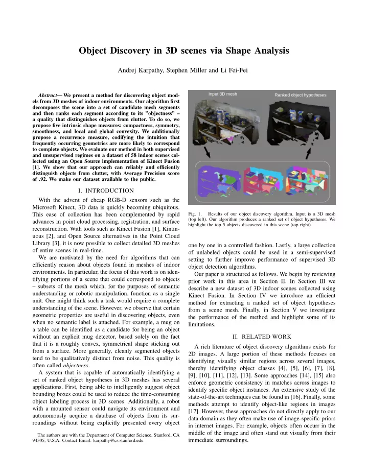
• Fig. 1.

Results of our object discovery algorithm. Input is a 3D mesh (top left). Our algorithm produces a ranked set of object hypotheses. We highlight the top 5 objects discovered in this scene (top right).

• ne by one in a controlled fashion. Lastly, a large collection
• f unlabeled objects could be used in a semi-supervised

setting to further improve performance of supervised 3D

• bject detection algorithms.

Our paper is structured as follows. We begin by reviewing prior work in this area in Section II. In Section III we describe a new dataset of 3D indoor scenes collected using Kinect Fusion. In Section IV we introduce an efficient method for extracting a ranked set of object hypotheses from a scene mesh. Finally, in Section V we investigate the performance of the method and highlight some of its limitations.

• II. RELATED WORK

A rich literature of object discovery algorithms exists for 2D images. A large portion of these methods focuses on identifying visually similar regions across several images, thereby identifying object classes [4], [5], [6], [7], [8], [9], [10], [11], [12], [13]. Some approaches [14], [15] also enforce geometric consistency in matches across images to identify specific object instances. An extensive study of the state-of-the-art techniques can be found in [16]. Finally, some methods attempt to identify object-like regions in images [17]. However, these approaches do not directly apply to our data domain as they often make use of image-specific priors in internet images. For example, objects often occurr in the middle of the image and often stand out visually from their immediate surroundings.

• Fig. 2.

Example scenes from our dataset.

Depth sensors have enabled approaches that reason about 3D shape of objects in a scene. [18], [19], [20] present algorithms for discovering visual categories in laser scans. A region-based approach is described in [21] that scores regions in a single RGB-D image according to a number of different shape and appearance cues. Recurrence has been used to discover objects in laser scans using RANSAC alignment [22]. Algorithms that identify objects based on changes in a scene across time have also been proposed [23], [24]. Our work is different from prior contributions in several

• respects. First, while prior work predominantly focuses on

single-view laser or RGB-D camera views, our input is a 3D mesh that is constructed from hundreds of overlap- ping viewpoints. Moreover, our focus is on realistic indoor environments that include variations in the type of scene, lighting conditions and the amount of clutter present. While

• bject recurrence has been shown to be a reliable cue, we
• bserve that many objects are relatively rare, and multiple,

identical instances are unlikely to be observed. And although motion can greatly aid in the segmentation task, many

• bjects are unlikely to be moved on a day-to-day level.

Therefore, in addition to a scene recurrence measure that leverages the intuitions of prior work, we propose a set of novel shape measures that evaluate a candidate segment’s shape to determine its objectness. Lastly, since our focus is on potentially large collections of scenes, our method is explicitly designed to be computationally efficient. Notably, this requires that we process scenes online one by one and in no particular order. While the core of the algorithm is fully unsupervised, we show how incorporating some supervision in form of object labels can further improve performance.

• III. DATASET GATHERING

Our dataset consists of 58 scenes recorded in the depart- ment offices, kitchens and printer rooms. We avoided manip- ulating the scenes prior to recording , to faithfully capture the complexities of the real world. As can be seen from Figure 2, our scenes can contain a significant amount of clutter and variation. Additionally, we collected the dataset during 6 different recording sessions to include variations with respect to lighting conditions (bright, dim, lights, natural light). In total, there are 36 office desks, 7 bookshelves, 4 printer room counters, 3 kitchens counters and 8 miscellaneous living space scenes. A significant portion of the objects in these scenes only occur once (roll of toilet paper, a chess set, a banana, an orange, a bag of coffee, etc.), while some objects

• ccur frequently (keyboards, mice, telephones, staplers, etc.).

The raw data for every scene consists of RGB-D video that ranges between 100 to 800 frames. During this time, an ASUS Xtion PRO LIVE RGB-D sensor is slowly moved around a part of a scene that contains structure. We use the

• pen source implementation of Kinect Fusion in the Point

Cloud Library [3] to process the videos into 3D colored meshes with outward-facing normals. The final result are 3D colored meshes with approximately 400,000 polygons and 200,000 vertices on average. These are available for download on the project website. 1

• IV. OBJECT DISCOVERY

We now describe in detail the steps of our discovery algorithm, as depicted in Figure 3. Inspired by previous work [21], [19], [22], our first step is to segment every scene into a set of mesh segments. Then, we consider every

1data and code are available at http://cs.stanford.edu/∼karpathy/discovery

segment individually as an object hypothesis and evaluate its

• bjectness according to a set of shape measures. Finally, the

measures for each segment are combined to give a score for its overall objectness.

• A. Scene Segmentation

The goal of the segmentation step is to identify plausible

• bject candidates in a scene. To partition a scene mesh into

segments, we treat the mesh as a graph and use a graph- based segmentation algorithm proposed by Felzenszwalb and Huttenlocher [25]. We experimented with several alternatives including normalized cuts and graph cuts, but settled on this

• ption because it produced good results at a low computa-

tional cost. Edge weights. The segmentation algorithm requires an edge weight to be specified between every pair of neighbor- ing points on the mesh. A natural choice is to consider the dot product between two normals ni, nj, but inspired by some prior work on segmentation in 3D scenes [26], we found that significantly more pleasing results can be obtained using a local curvature-aware metric. Intuitively, locally concave regions in the scene are more likely to correspond to object boundaries, while locally convex regions are likely to belong to an object and should not become segment boundaries. More precisely, we define point p j to be relatively convex to point pi if (pj − pi) · nj > 0, where n j is the normal at point pj. This predicate evaluates to true if the normal at pj points away from pi, which indicates that the surface is curving outwards. We compute the final edge weight (which can be interpreted as dissimilarity) as follows: wi j =

• (1−ni ·nj)2

if (pj − pi)·nj > 0 1−ni ·nj

• therwise

(1) Where the squared term serves to penalize convex edges less than concave edges. Note that a perfectly planar patch will produce edges with weight 0. We experimented with incorporating color into the sim- ilarity metric between points, but found that our attempts consistently lowered the overall performance of the system. We speculate that this could be due to significant lighting variations present in our dataset. More generally, we do not make use of color information throughout the algorithm, but still display colored meshes in figures for ease of interpreta- tion. Segment post-processing. Following the original imple- mentation of the graph segmentation algorithm, we place a hard threshold on the minimum number of points msize that are allowed to constitute a valid segment and greedily merge any smaller segments to neighboring segments. We use msize = 500, which with our data density corresponds to a shape about half the size of a computer mouse. Hard thresholding For added efficiency, we reject any segments that are more than 1m in size, or less than 2cm

• thin. In addition, denoting in decreasing order the eigenvalues
• f the scatter matrix as λ0,λ1,λ2 we also reject segments

that are, in relative terms, too thin ( λ1

λ0 < 0.05), or too flat

( λ2

λ0 < 0.001). These thresholds settings are conservative and

are not high enough to filter thin objects such as monitors. Non-maximum suppression Inevitably, some segments will be obtained multiple times across different settings of the segmentation algorithm’s granularity parameter. We detect such cases by computing intersection-over-union of vertices belonging to all segments. If two segments are found to be too similar (we use threshold of 0.7), we greedily retain the more object-like segment, computed as the average of the segment’s shape measures. We explain these measures next.

• Fig. 4.

Example of one of the segmentations of a scene. At this threshold, some objects are correctly identified while others, such as the headphones and monitor, are over-segmented.

• B. Objectness measures

Every segment identified during the segmentation step is evaluated using six objectness measures: five shape measures that are evaluated on every segment individually and a shape reccurrence measure. The recurrence measure is inspired by prior work [23], [22] that has identified repeated presence

• f a piece of geometry across space or time as evidence for
• bjectness. We now explain all measures in more detail.

Compactness rewards segments that contain structure in compact volume. Intuitively, this captures the bias of most

• bjects to being approximately spherical. We quantify this

notion by computing the ratio of the total surface area of the segment’s mesh to the surface area of its smallest bounding sphere.

• Symmetry. Objects often exhibit symmetries and their

role in visual perception has been explored in psychology [27]. Since the computational complexity of our method is a design consideration, we only consider evaluating reflective symmetry along the three principal axes of each segment. More specifically, we reflect the segment along a principal axis and measure the overlap between the original segment and its reflection. That is, denoting Λ = λx + λy + λz to be the sum of eigenvalues of the scatter matrix, and rx,ry,rz to be the extent of the segment along each of its principal axes, we calculate the symmetry of a cloud C as: Symmetry(C) =

∑

d∈{x,y,z}

λd Λ [(O(C,C−d,rd)+O(C−d,C,rd)] where C−d denotes reflection of cloud C along direction d. The one-sided overlap O between two clouds is calculated by summing up the difference in the position and direction of the normal from a point in one cloud to its nearest neighbor in the other:

• Fig. 3.

A visualization of our algorithm: every 3D input mesh is over-segmented into a large collection of segments. Each segment is ranked using our

• bjectness measures and the final ranking is computed. The last image highlights the top 5 objects found in the example scene.

O(C1,C2,r) = ∑

i=1..|C1|

1 r ||pC1

i − pC2 N(C2,pi)||+β(1−nC1 i ·nC2 N(C2,pi))

where pC

i denotes the i’th point in cloud C, similarly nC i

is the normal at point pi and N(C, p) evaluates to the index

• f the closest point to p in cloud C. Note that r is used to

normalize the distances based on the segment’s absolute size. Finally, β is a tunable parameter that trades off the relative importance of the two contributions (we use β = 0.2). Smoothness stipulates that every point on the mesh should have mass spread out uniformly around it. Intuitively, the presence of thin regions will cause a segment to score low, while neatly connected surfaces will score high. To compute the value of this measure at a single point p, we first project points in a local neighborhood around p to the tangent plane defined by its normal. Next, we quantize the angle of the projected points in the local 2D coordinate system into b bins and compute the entropy of the distribution. Here, high entropy indicates high smoothness. We repeat this procedure at each point and average the result across all points in the

• segment. In practice, we use b = 8 and local neighborhoods

with radius 1cm. Local Convexity. Surfaces of objects are often made up

• f locally convex regions. We determine the convexity of

each polygon edge as given by the predicate in Equation 1 and score each segment by the percentage of its edges which are convex. Global convexity. Visual perception studies have shown that the human visual system uses a global convexity prior when inferring 3D shape [28], [29]. Taking inspiration from these results, we also consider measuring the degree to which an object’s convex hull is an approximation to the

• bject’s shape. To evaluate this measure, we compute the

convex hull and record the average distance from a point on the object to the closest point on the convex hull.

• Recurrence. Segments that are commonly found in other

scenes are more likely to be an object rather than a seg- mentation artifact. Thus, for every segment we measure the average distance to the top k most similar segments in other

• scenes. In our experiments, we use k = 10.

There are several approaches one could use to quantify the distance between two segments. Prior work [22] has proposed computing local features on every object and using RANSAC followed by Iterative Closest Point algorithm to compute a rigid alignment. However, we found this strategy to be computationally too expensive. In Computer Vision, a standard approach is to compute visual bag of words representations from FPFH features [30] or spin images and match them using chi-squared kernels, but we found that while this approach gave reasonable results, it was also computationally too expensive. To keep the computational costs low, we found it is sufficient to retrieve segments of comparable sizes that have similar shape measures. Concretely, to retrieve the most similar segments to a given query segment, we consider all segments within 25% of extent along principal directions in size and measure the euclidean distance between their nor- malized shape measures. Each measure is normalized to be zero mean and unit variance during the retrieval. As a result,

• ur recurrence measure does not enforce exact alignment but

merely identifies segments that have commonly occurring statistical properties, as defined by our shape measures. Examples of nearest neighbor retrievals with this measure can be seen in figure 6.

• Fig. 6.

We show a query segment (left) and its 10 closest matches among all segments (right). These segments are retrieved from the entire set of 1836 segments across 58 scenes. Note that the third down are all cups, 5th row are all mice, and 8th row are mostly staplers.

• Fig. 5.

In every example scene above we highlight the top few object hypotheses, using the linear SVM as the predictor.

• C. Data-driven combination

We consider several options for combining the proposed measures into one objectness score: Simple averaging, Naive Bayes, Linear Support Vector Machine, RBF Kernel Support Vector Machine, and Nearest Neighbor. To obtain ground truth training labels, we manually an- notated all extracted segments as being an object or not. The labeling protocol we used is as follows. A segment is annotated as an object when it is an exact and full segmentation of a semantically interpretable part of the

• scene. If the segment contains surrounding clutter in addition

to the object, it is marked false. If a segment is only an object part that does not normally occur in the world in isolation, it is also marked false (for example, the top part of a stapler, the keypad on a telephone, the cover page of a book, etc.).

• V. RESULTS

We evaluated our method on the dataset described in Section III. Over-segmentation of all 58 scenes leads to a total of 1836 segments, of which we identified 303 as objects using the labeling protocol described in Section IV-C. We treat the task of identifying objects as a binary classification problem. To construct the data matrix we concatenate all measures into a 1836x6 matrix and normalize each column to be zero mean and unit variance. Next, we randomly assign half of the data to training set and half to the testing set. We perform 5-fold cross-validation on all classifier parameters using grid search. The entire process is repeated 20 times for different random splits of the data and the average result is reported. Quantitative analysis of the performance is shown in Figure 7. Example results for

• bject hypotheses can be seen visually in Figure 5.
• Limitations. The system is capable of reliably distin-

guishing objects once they are identified as potential object candidates, but there are a few common failure cases that cause the system to incorrectly miss an object candidate during the over-segmentation stage:

• 3D mesh reconstruction: A few failure cases are tied

directly to the mesh reconstruction step. Due to the limited resolution of Kinect Fusion’s volumetric rep- resentation, small neighboring objects may be fused together, causing the algorithm to undersegment these

• regions. Moreover, RGB-D sensors do not handle trans-

parent objects well, but transparent objects (bottles, plastic cups, glass tables) are relatively frequent in regular scenes. This can lead to noisy segments with large discontinuities in the reconstruction that cause

• ur algorithm to over-segment these regions. Lastly,

the resolution of the Marching Cubes reconstruction is limited by GPU memory. Low-resolution reconstruction can cause thin objects such as paper notebooks or thin keyboards to fuse into their supporting plane and not get discovered.

• Non-maximum suppression: An object part that occupies

a large fraction of the entire object can be judged by the algorithm to be much more object-like, which can cause the algorithm to incorrectly reject the entire object as a candidate. For instance, the two ear pieces of a pair of headphones tend to appear more objectlike in isolation than when connected by a thin plastic band.

• Fig. 7.

Precision vs. Recall curves for objectness measures and their combinations. Color-coded bar plots show Average Precisions.

Similarly, the cylindrical portion of a mug often appears more objectlike than it would with the handle attached.

• Segmentation algorithm: Our segmentation algorithm is

a compromise between speed and accuracy. Due to its limitations, it is particularly prone to over-segmenting extended objects that contain intricate structure. An example of such an object is a plant with many leaves. In addition, the segmentation algorithm will never consider joining two pieces that are not physically connected. For example, a transparent bottle with some liquid can easily become two disconnected segments: the body and the floating cap. As a result, the algorithm will never consider joining these segments into one candidate

• bject.

To estimate the extent of the problem quantitatively, we manually analyzed the recall of the system by counting the number of objects in each scene that should reasonably be identified as objects. We count on the order of 400 objects present in our dataset. Since we have 303 positive labels, we estimate the recall of the system to be roughly 75%. Figure 8 illustrates examples of failure cases visually. Quantitative analysis. As can be seen on Figure 7, the individual measures perform relatively poorly alone, but their combinations achieve impressive levels of performance. Moreover, it is interesting to note that even an unsupervised combination of our measures by means of simple averag- ing performs competitively: the top performer (RBF kernel SVM) achieves 0.92 Average Precision, while averaging achieves 0.86. We further seek to understand the contribution of indi- vidual measures by repeating the entire experiment with and without them. We use the RBF kernel SVM for these experiments as it has been shown to work best in our data. First, removing recurrence decreases performance of the system from 0.92 to 0.90 AP. Removing Symmetry, Local

• Fig. 8.

Examples of limitations. 1: Only main part of the headphones will be identified as a candidate object. 2: Cups are fused and get segmented together as a single object candidate. 3: The armrest of the chair will be incorrectly identified as a strong object. 4: Due to transparency, the top will appear to be floating and gets disconnected from the bottle. 5: The plant is too intricate and contains too much variation to be selected as a single

• bject. 6: The interior of the cup will be selected as a separate segment

because the curvature changes too quickly around its rim.

and Global Convexity similarly decrease performance by 2-3 points, but Compactness and Smoothness decrease the performance more significantly to 0.85 and 0.82 respectively. This hints that Compactness and Smoothness may be two of

• ur strongest measures. However, using Compactness and

Smoothness alone only achieves 0.81 AP, which indicates that the other measures still contribute meaningful informa- tion to the final result. Computational complexity. As motivated during the introduction, an important consid- eration for the design of our algorithm is its computational complexity.

• Fig. 9.

Confusion matrix for the RBF Kernel SVM.

Asymptotic analysis. Denoting N to be the number of scenes and S to be the average number of segments per scene (in this work N = 58 and S = 31), the complexity

• f the method is O(N) for mesh reconstruction, O(SN) to

evaluate the shape measures on all segments individually, and O((SN)2) to evaluate the recurrence measure. Even though a naive implementation of the recurrence measure is quadratic in the total number of segments, it is empirically the most efficient measure to compute on dataset of our size. Efficient k-nearest-neighbor algorithms such as FLANN [31] can be used to further speed up the retrieval process. Kinect Fusion. We computed the 3D meshes using the Open Source Kinect Fusion implementation [3] on an 8 core 2.2GHz laptop with the GTX 570m GPU. The process of converting the RGB-D video into 3D mesh took 2 minutes per scene on average. Measure computation. We further report computational time for an average scene with 200,000 vertices and 400,000 polygons on a 2.8GHz workstation, using a single-threaded implementation in C++:

Step Time(s) Over-segmentation 1.5 Compactness 0.1 Symmetry 3.8 Global Convexity 13.3 Local Convexity 1.3 Smoothness 2.5 Recurrence 0.1 Total 25

The entire 58 scene dataset can therefore be processed in about 25 minutes. As can be seen in the table above, the global convexity measure is by far the slowest step as it requires computing the convex hull.

• VI. CONCLUSION

We presented an approach for object discovery in a collec- tion of 3D meshes. Our algorithm is computationally efficient (running at about 25 seconds per scene on an average computer) and can process scenes independently and online. The core of the method relies on a set of proposed objectness measures that evaluate how likely a single mesh segment is to be an object. We demonstrated that these measures

can be averaged to reliably identify objects in scenes and showed that a supervised combination can further increase performance up to 0.92 Average Precision. We released a dataset of 58 challenging environments to the public. We estimated the overall recall of the system to be around 75% and qualitatively analyzed sources of error. The most common sources of error can be traced to limitations in data acquisition when dealing with transparent materials and the resolution of the resulting 3D mesh. While the simplicity of the segmentation algorithm allowed us to process scenes at very fast rates (segmenting an entire scene 10 times using different thresholds in 1.5 seconds), a more sophisticated formulation is necessary to ensure that complicated objects (such as the plant example in Figure 8) are segmented as a single candidate object. Future work includes increasing the recall of the system by improving the segmentation stage of the algorithm and by reasoning about segments in the context of the scene in which they were found. ACKNOWLEDGMENT This research is partially supported by an Intel ISTC research grant. Stephen Miller is supported by the Hertz Foundation Google Fellowship and the Stanford Graduate Fellowship. REFERENCES

[1] R. Newcombe, S. Izadi, O. Hilliges, D. Molyneaux, D. Kim, A. Davi- son, P. Kohli, J. Shotton, S. Hodges, and A. Fitzgibbon, “Kinectfusion: Real-time dense surface mapping and tracking,” in Mixed and Aug- mented Reality (ISMAR), 2011 10th IEEE International Symposium

• n.

IEEE, 2011, pp. 127–136. [2] T. Whelan, J. McDonald, M. Kaess, M. Fallon, H. Johannsson, and

• J. Leonard, “Kintinuous: Spatially extended KinectFusion,” in RSS

Workshop on RGB-D: Advanced Reasoning with Depth Cameras, Sydney, Australia, Jul 2012. [3] R. B. Rusu and S. Cousins, “3D is here: Point Cloud Library (PCL),” in IEEE International Conference on Robotics and Automation (ICRA), Shanghai, China, May 9-13 2011. [4] H. Arora, N. Loeff, D. Forsyth, and N. Ahuja, “Unsupervised seg- mentation of objects using efficient learning,” in Computer Vision and Pattern Recognition, 2007. CVPR’07. IEEE Conference on. IEEE, 2007, pp. 1–7. [5] M. Fritz and B. Schiele, “Decomposition, discovery and detection of visual categories using topic models,” in Computer Vision and Pattern Recognition, 2008. CVPR 2008. IEEE Conference on. IEEE, 2008,

• pp. 1–8.

[6] G. Kim, C. Faloutsos, and M. Hebert, “Unsupervised modeling of

• bject categories using link analysis techniques,” in Computer Vision

and Pattern Recognition, 2008. CVPR 2008. IEEE Conference on. IEEE, 2008, pp. 1–8. [7] B. Russell, W. Freeman, A. Efros, J. Sivic, and A. Zisserman, “Using multiple segmentations to discover objects and their extent in image collections,” in Computer Vision and Pattern Recognition, 2006 IEEE Computer Society Conference on, vol. 2. Ieee, 2006, pp. 1605–1614. [8] N. Payet and S. Todorovic, “From a set of shapes to object discovery,” Computer Vision–ECCV 2010, pp. 57–70, 2010. [9] J. Sivic, B. Russell, A. Efros, A. Zisserman, and W. Freeman, “Dis- covering objects and their location in images,” in Computer Vision,

• 2005. ICCV 2005. Tenth IEEE International Conference on, vol. 1.

Ieee, 2005, pp. 370–377. [10] J. Sivic, B. Russell, A. Zisserman, W. Freeman, and A. Efros, “Un- supervised discovery of visual object class hierarchies,” in Computer Vision and Pattern Recognition, 2008. CVPR 2008. IEEE Conference

• n.

IEEE, 2008, pp. 1–8. [11] M. Weber, M. Welling, and P. Perona, “Towards automatic discovery

• f object categories,” in Computer Vision and Pattern Recognition,
• 2000. Proceedings. IEEE Conference on, vol. 2.

IEEE, 2000, pp. 101–108. [12] I. Endres and D. Hoiem, “Category independent object proposals,” Computer Vision–ECCV 2010, pp. 575–588, 2010. [13] S. Vicente, C. Rother, and V. Kolmogorov, “Object cosegmentation,” in Computer Vision and Pattern Recognition (CVPR), 2011 IEEE Conference on. IEEE, 2011, pp. 2217–2224. [14] H. Kang, M. Hebert, and T. Kanade, “Discovering object instances from scenes of daily living,” in Computer Vision (ICCV), 2011 IEEE International Conference on. IEEE, 2011, pp. 762–769. [15] M. Cho, Y. Shin, and K. Lee, “Unsupervised detection and segmenta- tion of identical objects,” in Computer Vision and Pattern Recognition (CVPR), 2010 IEEE Conference on. IEEE, 2010, pp. 1617–1624. [16] T. Tuytelaars, C. Lampert, M. Blaschko, and W. Buntine, “Unsu- pervised object discovery: A comparison,” International journal of computer vision, vol. 88, no. 2, pp. 284–302, 2010. [17] B. Alexe, T. Deselaers, and V. Ferrari, “What is an object?” in Com- puter Vision and Pattern Recognition (CVPR), 2010 IEEE Conference

• n.

IEEE, 2010, pp. 73–80. [18] F. Endres, C. Plagemann, C. Stachniss, and W. Burgard, “Unsupervised discovery of object classes from range data using latent dirichlet allocation,” in Proc. of Robotics: Science and Systems, 2009. [19] R. Triebel, J. Shin, and R. Siegwart, “Segmentation and unsupervised part-based discovery of repetitive objects,” in Robotics: Science and Systems, vol. 2, 2010. [20] J. Shin, R. Triebel, and R. Siegwart, “Unsupervised 3d object dis- covery and categorization for mobile robots,” in Proc. of The 15th International Symposium on Robotics Research (ISRR), 2011. [21] A. Collet, S. Srinivasay, and M. Hebert, “Structure discovery in multi- modal data: a region-based approach,” in Robotics and Automation (ICRA), 2011 IEEE International Conference on. IEEE, 2011, pp. 5695–5702. [22] J. Shin, R. Triebel, and R. Siegwart, “Unsupervised discovery of repetitive objects,” in Robotics and Automation (ICRA), 2010 IEEE International Conference on. IEEE, 2010, pp. 5041–5046. [23] E. Herbst, P. Henry, X. Ren, and D. Fox, “Toward object discovery and modeling via 3-d scene comparison,” in Robotics and Automation (ICRA), 2011 IEEE International Conference on. IEEE, 2011, pp. 2623–2629. [24] E. Herbst, X. Ren, and D. Fox, “Rgb-d object discovery via multi- scene analysis,” in Intelligent Robots and Systems (IROS), 2011 IEEE/RSJ International Conference on. IEEE, 2011, pp. 4850–4856. [25] P. Felzenszwalb and D. Huttenlocher, “Efficient graph-based image segmentation,” International Journal of Computer Vision, vol. 59,

• no. 2, pp. 167–181, 2004.

[26] F. Moosmann, O. Pink, and C. Stiller, “Segmentation of 3d lidar data in non-flat urban environments using a local convexity criterion,” in Intelligent Vehicles Symposium, 2009 IEEE, june 2009, pp. 215 –220. [27] S. Palmer, “The role of symmetry in shape perception,” Acta Psycho- logica, vol. 59, no. 1, pp. 67–90, 1985. [28] M. Langer and H. Bulthoff, “A prior for global convexity in local shape-from-shading,” PERCEPTION-LONDON-, vol. 30, no. 4, pp. 403–410, 2001. [29] D. Kersten, P. Mamassian, and A. Yuille, “Object perception as bayesian inference,” Annu. Rev. Psychol., vol. 55, pp. 271–304, 2004. [30] R. B. Rusu, N. Blodow, and M. Beetz, “Fast point feature histograms (fpfh) for 3d registration,” in The IEEE International Conference

• n

Robotics and Automation (ICRA), Kobe, Japan, 05/2009 2009. [Online]. Available: http://files.rbrusu.com/publications/Rusu09ICRA.pdf [31] M. Muja and D. G. Lowe, “Fast approximate nearest neighbors with automatic algorithm configuration,” in International Conference on Computer Vision Theory and Application VISSAPP’09). INSTICC Press, 2009, pp. 331–340.