Numerical methods to overcome metastability in molecular dynamics - - PowerPoint PPT Presentation

Introduction Splitting strategies The Parallel Replica Algorithm Conclusion

Numerical methods to overcome metastability in molecular dynamics

• T. Lelièvre

CERMICS - Ecole des Ponts ParisTech & MicMac project-team - INRIA

Joint work with F. Cérou, A. Guyader, C. Le Bris, M. Luskin,

• D. Perez and D. Pommier. Special thanks to A. Voter.

Beyond Molecular Dynamics: Long Time Atomic-Scale Simulations March 2012

Introduction Splitting strategies The Parallel Replica Algorithm Conclusion

Introduction

The aim of molecular dynamics simulations is to understand the relationships between the macroscopic properties of a molecular system and its atomistic features. In particular, one would like to to evaluate numerically macroscopic quantities from models at the microscopic scale. Some examples of macroscopic quantities: (i) Thermodynamics quantities (average of some observable wrt an equilibrium measure): stress, heat capacity, free energy,... Eµ(ϕ(X )) =

• Rd ϕ(x) µ(dx).

(ii) Dynamical quantities (average over trajectories at equilibrium): diffusion coefficients, viscosity, transition rates,... E(F((X t)t≥0)) =

• C0(R+,Rd)

F((x t)t≥0)) W(d((x t)t≥0)).

Introduction Splitting strategies The Parallel Replica Algorithm Conclusion

Introduction

A molecular dynamics model amounts essentially in choosing a potential V which associates to a configuration (x1, ..., x N) = x ∈ R3N an energy V (x1, ..., x N). In the canonical (NVT) ensemble, configurations are distributed according to the Boltzmann-Gibbs probability measure: dµ(x) = Z −1 exp(−βV (x)) dx, where Z =

• exp(−βV (x)) dx is the partition function and

β = (kBT)−1 is proportional to the inverse of the temperature. Difficulties: (i) high-dimensional problem (N ≫ 1) ; (ii) µ is a multimodal measure.

Introduction Splitting strategies The Parallel Replica Algorithm Conclusion

Introduction

To sample µ, ergodic dynamics wrt to µ are used. A typical example is the over-damped Langevin (or gradient) dynamics: dX t = −∇V (X t) dt +

• 2β−1dW t.

It is the limit (when the mass goes to zero or the damping parameter to infinity) of the Langevin dynamics: ( dX t = M−1Pt dt, dPt = −∇V (X t) dt − γM−1Pt dt + p 2γβ−1dW t, where M is the mass tensor and γ is the friction coefficient.

To compute dynamical quantities, these are also typically the dynamics of interest. Thus, Eµ(ϕ(X)) ≃ 1 T T ϕ(X t) dt and E(F((X t)t≥0)) ≃ 1 N

N

• m=1

F((X m

t )t≥0).

In the following, we mainly consider the over-damped Langevin dynamics.

Introduction Splitting strategies The Parallel Replica Algorithm Conclusion

Introduction

Difficulty: In practice, X t is a metastable process, so that the convergence to equilibrium is very slow, and sampling metastable trajectories is very difficult. A 2d schematic picture: X 1

t is a slow variable (a metastable dof) of

the system. x1 x2 V (x1, x2) X 1

t

t

Introduction Splitting strategies The Parallel Replica Algorithm Conclusion

Introduction

Where does metastability come from ?

x coordinate y coordinate −1.5 −1 −0.5 0.5 1 1.5 −1.5 −1 −0.5 0.5 1 1.5 0.0 2000 4000 6000 8000 10000 −1.5 −1.0 −0.5 0.0 0.5 1.0 1.5

Time x coordinate

Energetic barrier.

x coordinate y coordinate

0.0 5000 10000 15000 20000 −8 −4 4 8

Time x coordinate

Entropic barrier.

Introduction Splitting strategies The Parallel Replica Algorithm Conclusion

Introduction

For computing thermodynamics quantities, there is a clear classification of available methods, and the difficulties are now well understood (in particular for free energy computations, see for example [TL, Rousset, Stoltz, 2010]). On the opposite, computing efficiently dynamical quantities remains a challenge. In this talk, we would like to discuss two methods to sample metastable dynamics and compute dynamical quantities:

• 1. Adaptive multilevel splitting method: A new algorithm related

to the forward flux sampling or the interface sampling method.

• 2. The Parallel Replica dynamics: An algorithm proposed by
• A. Voter in 1998 for which we propose a mathematical

analysis. There are many other techniques: hyperdynamics and temperature accelerated dynamics [Voter, Fichthorn], the string method [E, Ren,

Vanden-Eijnden], transition path sampling methods [Chandler, Bolhuis, Dellago],

milestoning techniques [Elber, Schuette, Vanden-Eijnden], etc...

Introduction Splitting strategies The Parallel Replica Algorithm Conclusion

Splitting strategies A B

Introduction Splitting strategies The Parallel Replica Algorithm Conclusion

Multilevel splitting

We would like to sample trajectories between two given metastable states A and B. The main assumption in this section is that we are given a smooth one dimensional function ξ : Rd → R (s.t. |∇ξ| = 0) which "indexes" the transition from A to B in the following sense: A ⊂ {x ∈ Rd, ξ(x) < zmin} and B ⊂ {x ∈ Rd, ξ(x) > zmax}, where zmin < zmax, and Σzmin (resp. Σzmax) is “close” to ∂A (resp. ∂B).

Example: ξ(x) = x −xA where xA ∈ A is a reference configuration in A.

Introduction Splitting strategies The Parallel Replica Algorithm Conclusion

Multilevel splitting

Question: How to compute dynamical quantities using ξ ? More precisely, we consider: (a) Reactive trajectories and (b) Transition times between the two metastable states A and B. We propose a multilevel splitting approach [Kahn, Harris, 1951] [Rosenbluth,

1955] to discard failed trajectories and branch trajectories

approaching the rare set. We focus on an adaptive variant [Cérou,

Guyader, 2007] [Cérou, Guyader, TL, Pommier, 2010]: the Adaptive Multilevel

Splitting (AMS) algorithm.

Introduction Splitting strategies The Parallel Replica Algorithm Conclusion

Reactive trajectory

A reactive trajectory between two metastable sets A and B is a piece of equilibrium trajectory that leaves A and goes to B without going back to A in the meantime [Hummer,2004] [Metzner, Schütte, Vanden-Eijnden,

2006].

A B

Difficulty: A trajectory leaving A is more likely to go back to A than to reach B.

Introduction Splitting strategies The Parallel Replica Algorithm Conclusion

AMS Algorithm

Initialisation: Generate an ensemble of N equilibrium trajectories starting from A, up to the time it reaches A or B, conditionnally to the fact that supt∈(0,τ n) ξ(X n

t ) > zmin. This is easily done by DNS.

Algorithm: (i) Order the zn = supt∈(0,τ n) ξ(X n

t ) ; (ii) Kill the

trajectory with the smallest supremum (say zn0) ; (iii) Create a new trajectory by branching another trajectory from the first time it crosses Σzn0 ; Go back to (i) until zn0 is larger than zmax. This generates an ensemble of N equilibrium trajectories starting from A, up to the time it reaches A or B, conditionnally to the fact that supt∈(0,τ n) ξ(X n

t ) > zmax.

Final step: To get reactive trajectories, one only retains paths which indeed end in B, and the part of the trajectory between A and B.

Remark: The algorithm can be seen as a kind of adaptive Forward Flux Sampling [Allen, Valeriani, Ten Wolde, 2009]. It is also related to the Interface Sampling Method [Bolhuis, van Erp, Moroni 2003] and the Milestoning method [Elber, Faradjian 2004]. See the review paper [Bolhuis, Dellago, 2009]

Introduction Splitting strategies The Parallel Replica Algorithm Conclusion

AMS Algorithm A B

Introduction Splitting strategies The Parallel Replica Algorithm Conclusion

AMS Algorithm A B

Introduction Splitting strategies The Parallel Replica Algorithm Conclusion

AMS Algorithm A B

Introduction Splitting strategies The Parallel Replica Algorithm Conclusion

AMS Algorithm A B

Introduction Splitting strategies The Parallel Replica Algorithm Conclusion

AMS Algorithm A B

Introduction Splitting strategies The Parallel Replica Algorithm Conclusion

AMS Algorithm A B

Introduction Splitting strategies The Parallel Replica Algorithm Conclusion

AMS Algorithm A B

Introduction Splitting strategies The Parallel Replica Algorithm Conclusion

AMS Algorithm

An important output of the algorithm is ˆ αN = (1 − 1/N)kmax r where N is the number of trajectories, kmax the number of iterations to reach the quantile zmax, and r the proportion of trajectories that do finally end in B and not in A (at the final step). The probability ˆ αN is an estimator of the probability for an equilibrium trajectory leaving A and reaching Σzmin to reach B before A. It may be interprated as a “probability of observing a reactive trajectory”. Values for ˆ αN in the numerical results below vary between 10−18 and 10−4 depending on the test cases: these are very rare events.

Introduction Splitting strategies The Parallel Replica Algorithm Conclusion

Numerical results

In all the numerical tests, we use overdamped dynamics, but the algorithm applies to any stochastic Markovian dynamics, is straightforward to parallelize, and requires only a small modification

• f an original MD code.

A 1D example: We consider the double-well potential: V (x) = x4 − 2x2, which has two minima at ±1 and one saddle point at 0. In this simple one dimensional setting, we set as metastable states A = {−1} and B = {+1}, and the reaction coordinate is taken to be simply ξ(x) = x. To test the consistency of the algorithm, we compute the distribution of the time-lengths of the reactive paths and compare to DNS (when possible).

Introduction Splitting strategies The Parallel Replica Algorithm Conclusion

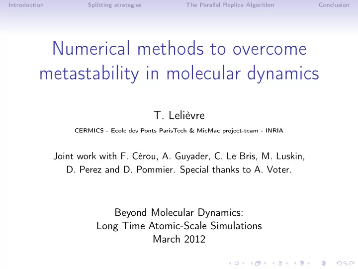
A 1D example

0.2 0.4 0.6 0.8 1 1.2 1.4 1.6 1.8 2 0.5 1 1.5 2 2.5 3 3.5 4 4.5 probability time Distribution of the length of a reactive path, beta=1 algorithm, 1E5 paths DNS, 1E5 paths 0.1 0.2 0.3 0.4 0.5 0.6 0.7 0.8 0.9 1 1 2 3 4 5 6 probability time Distribution of the length ofexpected time of a reactive path, beta=5 algorithm, 1E5 paths DNS, 1E5 paths 0.2 0.4 0.6 0.8 1 1.2 0.5 1 1.5 2 2.5 3 3.5 4 4.5 5 5.5 probability time Distribution of the length of a reactive path, beta=10 algorithm, 1E5 paths DNS, 1E4 paths 0.2 0.4 0.6 0.8 1 1.2 1.4 1.6 1.8 2 1 2 3 4 5 6 probability time Distribution of the length of a reactive path beta=1 beta=5 beta=10 beta=15 beta=20 beta=30 beta=40

Distributions of time-lengths of reactive paths. Comparison with DNS for β = 1, 5, 10 and distributions for β = 1, 5, 10, 15, 20, 30, 40.

Introduction Splitting strategies The Parallel Replica Algorithm Conclusion

A 1D example

β N ˆ αN DNS CPU AMS CPU 1 104 1.03 10−1 2s 2s 1 105 1.01 10−1 21s 1 min 19 s 10 104 2.04 10−5 140 min 05 s 5 s 10 105 1.98 10−5 1400 min ⋆ 5 min 22 s 15 105 1.78 10−7 92000 min ⋆ 7 min 52 s 20 105 1.33 10−9 8 min 36 s 40 105 5.82 10−18 10 min 09 s Probability ˆ αN, and computational time for different values of β and numbers of paths N. DNS CPU time with ⋆ is an extrapolated time deduced from a small number of generated reactive trajectories. The algorithm makes possible the generation of reactive trajectories for some parameter values for which DNS would be impractible.

Introduction Splitting strategies The Parallel Replica Algorithm Conclusion

A 2D example

Let us consider the potential ([Park, Sener, Lu, Schulten, 2003] [Metzner, Schütte and

Vanden-Eijnden, 2006]):

V (x, y) = 3e−x2−(y− 1

3)2 − 3e−x2−(y− 5 3)2 − 5e−(x−1)2−y 2

− 5e−(x+1)2−y 2 + 0.2x4 + 0.2

• y − 1

3 4 .

• 2
• 1.5
• 1
• 0.5

0.5 1 1.5 2

• 1.5
• 1
• 0.5

0.5 1 1.5 2 2.5

• 4
• 2

2 4 6 8 V(x,y) x y V(x,y)

Introduction Splitting strategies The Parallel Replica Algorithm Conclusion

A 2D example

The interest of this “bi-channel” potential is that, depending on the temperature, one or the other channel is prefered to go from A (around H− = (−1, 0)) to B (around H+ = (1, 0)). We will look at two quantities ([Hummer,2004] [Metzner, Schütte, Vanden-Eijnden,

2006]): the density of configurations along reactive paths, and the

flux of reactive trajectories, for two values of the inverse temperature β = 1.67 and β = 6.67. Two reaction coordinates are tested: ξ1(x, y) = x or ξ2(x, y) = (x, y) − H−. Both give reliable results, even though: (i) They are not the commitor functions ; (ii) The system exhibits metastabilities at fixed values of ξi.

Introduction Splitting strategies The Parallel Replica Algorithm Conclusion

Density on reactive paths

• 1.2
• 0.6

0.6 1.2

• 1
• 0.25

0.5 1.25 2. 5e-05 0.0001 0.00015 0.0002 0.00025 0.0003 0.00035 Density for beta = 1.67 x y 5e-05 0.0001 0.00015 0.0002 0.00025 0.0003 0.00035

• 1.2
• 0.6

0.6 1.2

• 1
• 0.25

0.5 1.25 2. 0.0005 0.001 0.0015 0.002 0.0025 0.003 0.0035 0.004 Density for beta = 6.67 x y 0.0005 0.001 0.0015 0.002 0.0025 0.003 0.0035 0.004

Results obtained for ξ1(x, y) = x and N = 105. Left: β = 1.67 ; Right: β = 6.67.

Introduction Splitting strategies The Parallel Replica Algorithm Conclusion

Density on reactive paths

• 1.2
• 0.6

0.6 1.2

• 1
• 0.25

0.5 1.25 2. 5e-05 0.0001 0.00015 0.0002 0.00025 0.0003 0.00035 0.0004 Density for beta = 1.67 x y 5e-05 0.0001 0.00015 0.0002 0.00025 0.0003 0.00035 0.0004

• 1.2
• 0.6

0.6 1.2

• 1
• 0.25

0.5 1.25 2. 0.0005 0.001 0.0015 0.002 0.0025 0.003 0.0035 0.004 Density for beta = 6.67 x y 0.0005 0.001 0.0015 0.002 0.0025 0.003 0.0035 0.004

Results obtained for ξ2(x, y) = (x, y) − H− and N = 105. Left: β = 1.67 ; Right: β = 6.67.

Introduction Splitting strategies The Parallel Replica Algorithm Conclusion

Density on reactive paths

• 1.2
• 0.6

0.6 1.2

• 1
• 0.25

0.5 1.25 2. 5e-05 0.0001 0.00015 0.0002 0.00025 0.0003 0.00035 0.0004 Density for beta = 1.67 x y 5e-05 0.0001 0.00015 0.0002 0.00025 0.0003 0.00035 0.0004

• 1.2
• 0.6

0.6 1.2

• 1
• 0.25

0.5 1.25 2. 0.0005 0.001 0.0015 0.002 0.0025 0.003 0.0035 0.004 Density for beta = 6.67 x y 0.0005 0.001 0.0015 0.002 0.0025 0.003 0.0035 0.004

Results obtained for ξ2(x, y) = (x, y) − H− and N = 104. Left: β = 1.67 ; Right: β = 6.67.

Introduction Splitting strategies The Parallel Replica Algorithm Conclusion

Flux of reactive trajectories

• 1
• 0.5

0.5 1 1.5

• 1
• 0.5

0.5 1 y x Flux of reactive path 0.2 0.4 0.6 0.8 1

• 0.5

0.5 1 1.5 2

• 1
• 0.5

0.5 1 y x Flux of reactive path 0.2 0.4 0.6 0.8 1

• 0.5

0.5 1 1.5 2

• 1
• 0.5

0.5 1 0.2 0.4 0.6 0.8 1

• 0.5

0.5 1 1.5 2

• 1
• 0.5

0.5 1 0.2 0.4 0.6 0.8 1

Flux of reactive trajectories, at β = 1.67 on the left, and β = 6.67

• n the right.

Introduction Splitting strategies The Parallel Replica Algorithm Conclusion

Computing transition times

To use the algorithm to compute transition times, we split a transition path from A to B into: excursions from ∂A to Σzmin and then back to ∂A, and finally an excursion from ∂A to Σzmin and then to B. Assuming Σzmin is close to an iso-commitor (Markov property), one obtains that the mean transition time is: E(T) = 1 p − 1

• E(T1 + T2) + E(T1 + T3)

where:

• p is the probability, once Σzmin has been reached, to go to B

rather than A (approximated by ˆ αN) ;

• E(T1 + T2) is the mean time for an excursion from ∂A to

Σzmin and then back to ∂A (approximated by DNS) ;

• E(T1 + T3) is the mean time for an excursion from ∂A to

Σzmin and then to B (approximated by the AMS algorithm).

Introduction Splitting strategies The Parallel Replica Algorithm Conclusion

Numerical results

Numerical results on the 1D case β ∆t zmin E(T) E(T) C.I. in E(T) Error (DNS) (AMS) (AMS) (%) 5 0.010 −0.9 185 208.3 [199.6, 217.7] 12.591 5 0.010 −0.6 185 221.2 [214.3, 228.4] 19.577 5 0.001 −0.9 185 187.4 [180.5, 194.8] 1.292 5 0.001 −0.6 185 193.2 [188.3, 198.3] 4.459 7 0.010 −0.9 1405 1515 [1468, 1565] 7.832 7 0.010 −0.6 1405 1642 [1567, 1722] 16.847 7 0.001 −0.9 1405 1380 [1316, 1449] 1.808 7 0.001 −0.6 1405 1400 [1358, 1444] 0.370 Transition times for small values of β, with various time steps ∆t and zmin. Reference values are computed by DNS.

Introduction Splitting strategies The Parallel Replica Algorithm Conclusion

Numerical results

5 10 15 20 25 30 35 40 45 5 10 15 20 25 30 35 40 time, log-scale beta y=x

Comparison of the estimated mean transition times as a function of β with the asymptotic law from large deviation theory: E(T) ∝ exp(β∆V ) where ∆V = 1 is the height of the energy barrier.

Introduction Splitting strategies The Parallel Replica Algorithm Conclusion

Numerical results

Numerical results on the 2D case N β kAB C.I. on kAB ×103 (AMS) (AMS) 2 1.67 2.03 10−2 [1.83; 2.22] 10−2 10 1.67 1.84 10−2 [1.82; 1.86] 10−2 50 1.67 1.88 10−2 [1.87; 1.88] 10−2 100 1.67 1.89 10−2 [1.89; 1.90] 10−2 2 6.67 9.97 10−8 [7.74; 12.2] 10−8 10 6.67 9.20 10−8 [7.71; 10.7] 10−8 50 6.67 8.88 10−8 [8.42; 9.34] 10−8 100 6.67 9.32 10−8 [9.08; 9.57] 10−8 Estimates of the reaction rate kAB = 2/E(T), withξ = ξ2. Values from [Metzner, Schütte, Vanden-Eijnden, 2006] are kAB = 1.912 10−2 for β = 1.67 and kAB = 9.47 10−8 for β = 6.67.

Introduction Splitting strategies The Parallel Replica Algorithm Conclusion

Adaptive multilevel splitting: conclusions

Possible extensions:

• Generate equilibrium trajectories which leave a metastable

state A without knowing the neighborhood.

• Adaptively compute a better and better ξ (proportional to the

committor function). The mathematical analysis of the AMS algorithm remains essentially to be done:

• Analysis of the time discretization error,
• Asymptotic variance of the estimator and optimization of ξ,
• Precise estimate of the bias.

Introduction Splitting strategies The Parallel Replica Algorithm Conclusion

The Parallel Replica Algorithm

Introduction Splitting strategies The Parallel Replica Algorithm Conclusion

The Parallel Replica Algorithm

The Parallel Replica Algorithm, proposed by A.F. Voter in 1998, is a method to get efficiently a "coarse-grained projection" of a dynamics. Let us consider again the overdamped Langevin dyanmics: dX t = −∇V (X t) dt +

• 2β−1dW t

and let assume that we are given a smooth mapping S : Rd → N which to a configuration in Rd associates a state number. Think of a numbering of the wells of the potential V . The aim of the parallel replica dynamics is to generate very efficiently a trajectory (St)t≥0 which has (almost) the same law as (S(X t))t≥0.

Introduction Splitting strategies The Parallel Replica Algorithm Conclusion

The Parallel Replica Algorithm

Initialization: Consider an initial condition X ref for a reference walker, the associated initial condition S0 = S(X ref

0 ), and a

simulation time counter Tsimu = 0. Then, one iteration of the algorithm goes through three steps.

• The decorrelation step: Let the reference walker (X ref

Tsimu+t)t≥0

evolve over a time interval t ∈ [0, τcorr]. Then,

• If the process leaves the well during the time interval (i.e.

∃t ≤ τcorr such that S

• X ref

Tsimu+t

• = S
• X ref

Tsimu

• ) advance the

simulation clock by τcorr and restart the decorrelation step ;

• otherwise, advance the simulation clock by τcorr and proceed

to the dephasing step.

During all this step, STsimu+t := S

• X ref

Tsimu+t

• .

Introduction Splitting strategies The Parallel Replica Algorithm Conclusion

The Parallel Replica Algorithm

The reference walker enters a new state

Introduction Splitting strategies The Parallel Replica Algorithm Conclusion

The Parallel Replica Algorithm

Decorrelation step: wait for a time τcorr.

Introduction Splitting strategies The Parallel Replica Algorithm Conclusion

• The dephasing step: Duplicate the walker X ref

Tsimu into N

• replicas. Let these replicas evolve independently and in parallel
• ver a time interval of length τdephase. If a replica leaves the

well during this time interval, restart the dephasing step for this replica. Throughout this step, the simulation counter is stopped.

Introduction Splitting strategies The Parallel Replica Algorithm Conclusion

The Parallel Replica Algorithm

Dephasing step.

Introduction Splitting strategies The Parallel Replica Algorithm Conclusion

The Parallel Replica Algorithm

Dephasing step: generate new initial conditions in the state.

Introduction Splitting strategies The Parallel Replica Algorithm Conclusion

The Parallel Replica Algorithm

Dephasing step: generate new initial conditions in the state.

Introduction Splitting strategies The Parallel Replica Algorithm Conclusion

The Parallel Replica Algorithm

Dephasing step: generate new initial conditions in the state.

Introduction Splitting strategies The Parallel Replica Algorithm Conclusion

The Parallel Replica Algorithm

Dephasing step: generate new initial conditions in the state.

Introduction Splitting strategies The Parallel Replica Algorithm Conclusion

The Parallel Replica Algorithm

Dephasing step: generate new initial conditions in the state.

Introduction Splitting strategies The Parallel Replica Algorithm Conclusion

The Parallel Replica Algorithm

Dephasing step: generate new initial conditions in the state.

Introduction Splitting strategies The Parallel Replica Algorithm Conclusion

The Parallel Replica Algorithm

Dephasing step: generate new initial conditions in the state.

Introduction Splitting strategies The Parallel Replica Algorithm Conclusion

• The parallel step: Let all the replicas evolve independently and

track the first escape event: T = inf

k T k W = T K0 W

where K0 = arg infk T k

W and

T k

W = inf{t ≥ 0, S(X k Tsimu+t) = S(X k Tsimu)}

is the first time the k-th replica leaves the well. Then: Tsimu = Tsimu + NT and X ref

Tsimu+NT = X K0 Tsimu+T.

Moreover, over [Tsimu, Tsimu + NT], the state dynamics St is constant and defined as: St = S(X 1

Tsimu).

Then, go back to the decorrelation step...

Introduction Splitting strategies The Parallel Replica Algorithm Conclusion

The Parallel Replica Algorithm

Parallel step.

Introduction Splitting strategies The Parallel Replica Algorithm Conclusion

The Parallel Replica Algorithm

Parallel step: run independent trajectories in parallel...

Introduction Splitting strategies The Parallel Replica Algorithm Conclusion

The Parallel Replica Algorithm

Parallel step: ... and detect the first transition event.

Introduction Splitting strategies The Parallel Replica Algorithm Conclusion

The Parallel Replica Algorithm

Parallel step: update the time clock: Tsimu = Tsimu + NT.

Introduction Splitting strategies The Parallel Replica Algorithm Conclusion

The Parallel Replica Algorithm

A new decorrelation step starts...

Introduction Splitting strategies The Parallel Replica Algorithm Conclusion

The Parallel Replica Algorithm

New decorrelation step

Introduction Splitting strategies The Parallel Replica Algorithm Conclusion

The Parallel Replica Algorithm

Analysis of the algorithm: the parallel step would introduce no error if

• the escape time T 1

W was exponentially distributed

• and independent of the next visited state.

This essentially amounts to assuming that S(X t) is a Markov chain... How to analyze the error introduced by the algorithm ? This is related to the general question: how to relate a continuous state space Markov dynamics to a discrete state space Markov dynamics ? Pitfalls: (i) the temperature is not necessarily small (ii) the

partition of the state space may be anything (iii) no thermodynamic limit in general (non-homogeneous systems).

Introduction Splitting strategies The Parallel Replica Algorithm Conclusion

The quasi-stationary distribution

The quasi-stationary distribution (QSD) ν for X t and associated to the actual well W is a probability measure which is (i) supported by W and such that (ii): ∀t > 0, ∀A ⊂ W , ν(A) =

• W

P(X x

t ∈ A, t < T x W ) ν(dx)

• W

P(t < T x

W ) ν(dx)

. If X 0 ∼ ν and if (X s)0≤s≤t has not left the well, then X t ∼ ν. Let L = −∇V · ∇ + β−1∆ be the infinitesimal generator of (X t). Then the density u of ν (dν = u(x)dx) is the first eigenfunction of L∗ = div (∇V + β−1∇) with absorbing boundary conditions:

• L∗u = −λ1u on W ,

u = 0 on ∂W .

Introduction Splitting strategies The Parallel Replica Algorithm Conclusion

The quasi-stationary distribution and the dephasing step

Property of the QSD: If X 0 ∼ ν then, the first exit time TW from W is exponentially distributed with parameter λ1 and is a random variable independent of the first hitting point X TW on ∂W . The dephasing step is very much related to the so-called Fleming-Viot process and may be seen as a way to get N i.i.d. random variables distributed according to the QSD. Remark: In general, TW exponentially distribtued is not sufficient for X 0 to be distributed according to ν.

Introduction Splitting strategies The Parallel Replica Algorithm Conclusion

The parallel step

As announced above, starting from the QSD, the parallel step is

• exact. This is stated precisely here.

Let us start from N initial conditions X k

0 i.i.d. in the well W and

let the processes evolve independently. Let us denote T k

W = inf{t > 0, X k t ∈ W }

the escape time for the k-th replica, and T = T K0

W where K0 = arg

min

k∈{1,...,N} T k W

the first escape time over all processes.

• Assume that T 1

W is exponentially distributed [OK starting

from QSD.] Then NT has the same law as T 1

W .

• Assume that T 1

W is independent of X 1 T 1

W [OK starting from

QSD.] Then X K0

T K0

W

has the same distribution as X 1

T 1

W and is

independent of T K0

W .

Introduction Splitting strategies The Parallel Replica Algorithm Conclusion

The decorrelation step

We would like to quantify the error introduced by the dephasing and parallel steps, when the decorrelation step is successful. As shown above, when the decorrelation step is successful, it is assumed that the reference walker is distributed according to the

• QSD. If it was indeed the case, the algorithm would be exact. The

decorrelation step can be seen as a way to probe this assumption. What is the error introduced there ?

Introduction Splitting strategies The Parallel Replica Algorithm Conclusion

The decorrelation step

We have the following error estimate in total variation norm: for t ≥

C λ2−λ1 ,

sup

f ,f L∞ ≤1

• E(f (TW −t, X TW )|TW ≥ t)−Eν(f (TW , X TW ))
• ≤ C exp(−(λ2−λ1)t),

where −λ2 < −λ1 < 0 are the two first eigenvalues of L∗ with absorbing boundary conditions on ∂W . This shows that τcorr should be chosen such that: τcorr ≥ C λ2 − λ1 . On the other hand, it should be smaller than the typical time to leave the well, E(TW ). Since Eν(TW ) = 1/λ1, this typically implies the spectral gap requirement, C λ2 − λ1 ≤ 1 λ1 .

Introduction Splitting strategies The Parallel Replica Algorithm Conclusion

The Parallel Replica Algorithm: conclusions

This can be generalized to other dynamics (coarse-graining of kMC). Main results:

• The QSD is a good intermediate between continuous state

dynamics and kMC-like approximations.

• The error analysis holds whatever the partition. But the

method requires metastability between the states to be computationally efficient.

• The parameter τcorr should be adjusted in terms of the two

first eigenvalues of the Fokker-Planck operator with absorbing boundary conditions.

Introduction Splitting strategies The Parallel Replica Algorithm Conclusion

Conclusion

Notice that the numerical methods we have presented are based on some dimension reduction and coarse-graining techniques (through the functions ξ or S). They are easy to parallelize.

Introduction Splitting strategies The Parallel Replica Algorithm Conclusion

Conclusion

A few references:

• F. Cérou, A. Guyader, T. Lelièvre and D. Pommier, A multiple

replica approach to simulate reactive trajectories, Journal of Chemical Physics 134, 054108, 2011.

• T. Lelièvre, M. Rousset and G. Stoltz, Free energy computations, a

mathematical perspective, Imperial College Press, 2010.

• C. Le Bris, T. Lelièvre, M. Luskin and D. Perez, A mathematical

formalization of the parallel replica dynamics, http://arxiv.org/abs/1105.4636, to appear in Monte Carlo Methods and Applications.