SLIDE 1 Numerical differentiation!
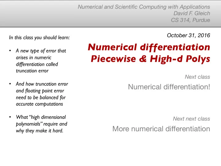
Numerical and Scientific Computing with Applications David F . Gleich CS 314, Purdue October 31, 2016
Numerical differentiation Piecewise & High-d Polys
Next class
More numerical differentiation
Next next class In this class you should learn:
arises in numeric differentiation called truncation error
and floating point error need to be balanced for accurate computations
polynomials” require and why they make it hard.
SLIDE 2
Piecewise polynomial approximation
Used all over!
SLIDE 3
Powerpoint curves
SLIDE 4
Piecewise polynomial approximation
a
SLIDE 5
Piecewise polynomial approximation
SLIDE 6
f(x2) f(x1) f(x3) f(x4) f(x5) x1 x2 x3 x4 x5
`(x) = f(xi−1) x − xi xi−1 − xi + f(xi) x − xi−1 xi − xi−1
In each subinterval
SLIDE 7
f(x2) f(x1) f(x3) f(x4) f(x5) x1 x2 x3 x4 x5
`(x) = f(xi−1) x − xi xi−1 − xi + f(xi) x − xi−1 xi − xi−1
In each subinterval
SLIDE 8
Piecewise polynomial approximation
Linear Uses a set of functions values & points
Good if there are many points
Quadratic Same info
Can use extra point to match midpoints
Cubic Hermite Uses points, function values, and derivatives
Matches the function values and derivatives!
Cubic Splines Uses points, function values
A twice continuously differentiable interpolant!
SLIDE 9
Piecewise polynomial approximation
Linear Easy! Quadratic Easy! Cubic Hermite Local work Cubic Splines Global work
`(x) = f(xi−1) x − xi xi−1 − xi + f(xi) x − xi−1 xi − xi−1
SLIDE 10
Cubic Hermite
4 parameters, 4 unknowns in the cubic polynomial between xi, xi+1 Fit via differentiation. One continuous derivative! See the book.
xi xi+1
f(xi) f’(xi) f(xi+1) f’(xi+1)
SLIDE 11
Cubic Splines
4(n-1) parameters, e.g. 4 unknowns in the cubic polynomial between xi, xi+1 Matching points gives 2(n-1) constraints Derivatives are continuous (n-3) constraints 2nd derivatives are continuous (n-3) constraints
x3 x4
f(xi) f(xi+1)
x2 x1
SLIDE 12 Cubic Splines
x3 x4
f(xi) f(xi+1)
x2 x1
α1 β1 β1 α2 β2 β2 ... ... ... ... βn−2 βn−2 αn−1 z1 z2 . . . . . . zn−1 = b1 b2 . . . . . . bn−1
s00
i (x) = zi1
x − xi xi1 − xi + zi x − xi1 xi − xi1
Piecewise linear second derivative Continuous derivative gives us a linear system
SLIDE 13 Multivariate functions
−5 5 −5 5 0.2 0.4 0.6 0.8 1 x y
f(x, y) = 1 1 + x2 + y2
SLIDE 14
Multivariate polynomials
A bi-variate (2 variable) quadratic has 9 unknown parameters A bi-variate (2 variable) cubic has 16 unknown parameters A tri-variate (3 variable) quadratic has 27 unknown parameters A tri-variate (3 variable) cubic has ? unknown parameters
f(x, y) = c2,2x2y2 + c1,2xy2 + c0,2y2 + c2,1x2y + c1,1xy + c0,1y + c2,0x2 + c1,0x + c0,0
SLIDE 15
Degree of multivariate polynomials
x2 y2 has degree “four” x y2 has degree “three” the degree of a multivar poly is the degree of the largest term
f(x, y) = c2,2x2y2 + c1,2xy2 + c0,2y2 + c2,1x2y + c1,1xy + c0,1y + c2,0x2 + c1,0x + c0,0
f(x, y) = c0,2y2 + + c1,1xy + c0,1y + c2,0x2 + c1,0x + c0,0
SLIDE 16
Quiz
Write down the equations for a multi-linear function in three dimensions: (1) where all degrees are less than or equal to 1 (2) where all “linear” terms of present
f(x, y) = c2,2x2y2 + c1,2xy2 + c0,2y2 + c2,1x2y + c1,1xy + c0,1y + c2,0x2 + c1,0x + c0,0
f(x, y) = c0,2y2 + + c1,1xy + c0,1y + c2,0x2 + c1,0x + c0,0
SLIDE 17 Fitting multivariate polynomials
… not nice to write down in general …
- Saniee. “A simple form of the multivariate Lagrange interpolant”
SIAM J. Undergraduate Research Online, 2007.
f(x, y) = c0,2y2 + + c1,1xy + c0,1y + c2,0x2 + c1,0x + c0,0
SLIDE 18 An easier special case
If we have data from
repeated grid then we can fit a sum of 1d polynomials “tensor product constructions”
x1 x2 x3 x4 x5 x6 y1 y2 y3 y4 y5 y6 y7
p(x, y) = X zijϕx
i (x)ϕy j (y)
SLIDE 19
The big problem
If we have an m dimensional function And we want an n degree interpolant We need (n+1)m samples of our function. “quadratic” in 10 dimensions – 310 samples “quadratic” in 100 dimensions – 3100 samples Exponential growth or “curse of dimensionality”
SLIDE 20
Quiz
Write down the equations for a linear interpolant in three dimensions: (1) where all degrees are less than 1 (2) where all “linear” terms of present
SLIDE 21
Polynomial approximation
Chebfun implements 1d polynomial interpolation, just use it! Equally spaced points are bad for interpolation! There are many mathematically equivalent variations on unique polynomial interpolants but they have different computation properties Piece-wise polynomials are a highly-flexible model for modeling general smooth curves. High dimensional interpolation is really hard