
SLIDE 1
CIS 541 - Differentiation
Roger Crawfis
August 12, 2005 OSU/CIS 541 2
Numerical Differentiation
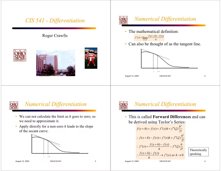
- The mathematical definition:
- Can also be thought of as the tangent line.
( ) ( ) '( ) lim
h
f x h f x f x h
→
+ − =
x x+h
August 12, 2005 OSU/CIS 541 3
Numerical Differentiation
- We can not calculate the limit as h goes to zero, so
we need to approximate it.
- Apply directly for a non-zero h leads to the slope
- f the secant curve.
x x+h
August 12, 2005 OSU/CIS 541 4
Numerical Differentiation
- This is called Forward Differences and can
be derived using Taylor’s Series:
2 2