Nuclear Chart Periodic Table of the Elements Group** Period 1 18 - - PDF document

nuclear chart
SMART_READER_LITE
LIVE PREVIEW

Nuclear Chart Periodic Table of the Elements Group** Period 1 18 - - PDF document

Takashi NAKATSUKASA Theoretical Nuclear Physics Laboratory RIKEN Nishina Center Real-space, real-time approaches DFT, TDDFT ((Q)RPA ) Few-body model (CDCC )


slide-1
SLIDE 1

計算核データ 構築に向けて

Takashi NAKATSUKASA Theoretical Nuclear Physics Laboratory RIKEN Nishina Center

2009.3.25-26 Mini-WS:核データ と 核理論

  • Real-space, real-time approaches

→ DFT, TDDFT ((Q)RPAと 相補的) Few-body model (CDCCと 相補的)
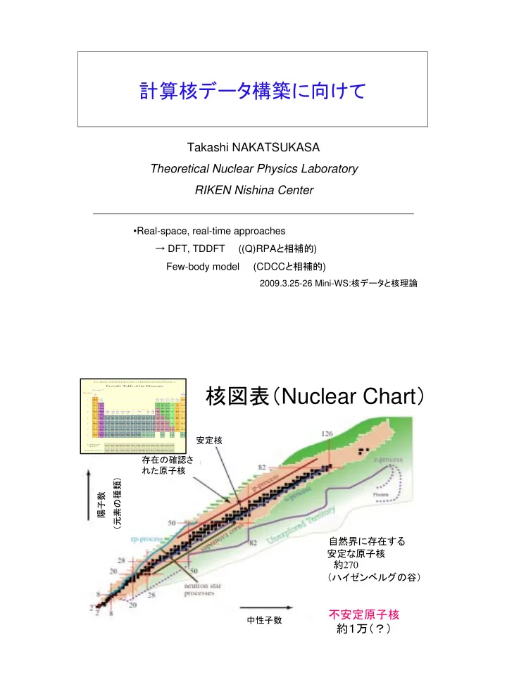
核図表( Nuclear Chart)

自然界に存在する 安定な原子核 約270 ( ハイ ゼンベルグの谷)

不安定原子核 約1 万( ?)

中性子数 陽子数 ( 元素の種類) 安定核 存在の確認さ れた原子核

Los Alamos National Laboratory's Chemistry Division Presents a

Periodic Table of the Elements

Group** Period

1 IA 1A 18 VIIIA 8A 1 1

H

1.008 2 IIA 2A 13 IIIA 3A 14 IVA 4A 15 VA 5A 16 VIA 6A 17 VIIA 7A 2

He

4.003 2 3

Li

6.941 4

Be

9.012 5

B

10.81 6

C

12.01 7

N

14.01 8

O

16.00 9

F

19.00 10

Ne

20.18 8 9 10 3 11

Na

22.99 12

Mg

24.31 3 IIIB 3B 4 IVB 4B 5 VB 5B 6 VIB 6B 7 VIIB 7B
  • ------ VIII -----
  • ------ 8 -------
11 IB 1B 12 IIB 2B 13

Al

26.98 14

Si

28.09 15

P

30.97 16

S

32.07 17

Cl

35.45 18

Ar

39.95 4 19

K

39.10 20

Ca

40.08 21

Sc

44.96 22

Ti

47.88 23

V

50.94 24

Cr

52.00 25

Mn

54.94 26

Fe

55.85 27

Co

58.47 28

Ni

58.69 29

Cu

63.55 30

Zn

65.39 31

Ga

69.72 32

Ge

72.59 33

As

74.92 34

Se

78.96 35

Br

79.90 36

Kr

83.80 5 37

Rb

85.47 38

Sr

87.62 39

Y

88.91 40

Zr

91.22 41

Nb

92.91 42

Mo

95.94 43

Tc

(98) 44

Ru

101.1 45

Rh

102.9 46

Pd

106.4 47

Ag

107.9 48

Cd

112.4 49

In

114.8 50

Sn

118.7 51

Sb

121.8 52

Te

127.6 53

I

126.9 54

Xe

131.3 6 55

Cs

132.9 56

Ba

137.3 57

La*

138.9 72

Hf

178.5 73

Ta

180.9 74

W

183.9 75

Re

186.2 76

Os

190.2 77

Ir

190.2 78

Pt

195.1 79

Au

197.0 80

Hg

200.5 81

Tl

204.4 82

Pb

207.2 83

Bi

209.0 84

Po

(210) 85

At

(210) 86

Rn

(222) 7 87

Fr

(223) 88

Ra

(226) 89

Ac~

(227) 104

Rf

(257) 105

Db

(260) 106

Sg

(263) 107

Bh

(262) 108

Hs

(265) 109

Mt

(266) 110
  • ()
111
  • ()
112
  • ()
114
  • ()
116
  • ()
118
  • ()
Lanthanide Series* 58

Ce

140.1 59

Pr

140.9 60

Nd

144.2 61

Pm

(147) 62

Sm

150.4 63

Eu

152.0 64

Gd

157.3 65

Tb

158.9 66

Dy

162.5 67

Ho

164.9 68

Er

167.3 69

Tm

168.9 70

Yb

173.0 71

Lu

175.0 Actinide Series~ 90

Th

232.0 91

Pa

(231) 92

U

(238) 93

Np

(237) 94

Pu

(242) 95

Am

(243) 96

Cm

(247) 97

Bk

(247) 98

Cf

(249) 99

Es

(254) 100

Fm

(253) 101

Md

(256) 102

No

(254) 103

Lr

(257)
slide-2
SLIDE 2

High-performance computing ~ DFT to cover all

One-to-one Correspondence

External potential Ground state Density

v-representative density

Minimum-energy state

( )

r

V

r ρ

V

Ψ ) (r V r

( )

r r ρ Ψ

slide-3
SLIDE 3

[ ]

( ) { } 0

) ( ) ( ) ( = − − +

∫ ∫

N r d r r d r v r F r r r r r ρ µ ρ ρ δ

The following variation leads to all the ground-state properties. In principle, any physical quantity of the ground state should be a functional of density. Variation with respect to many-body wave functions ↓ Variation with respect to one-body density ↓ Physical quantity

) , , ( 1

N

r r r L r Ψ

) (r r ρ ] [ ˆ ] [ )] ( [ ρ ρ ρ Ψ Ψ = A r A r

Kohn-Sham Scheme

Ground state

density

( )

r r ρ

V

Ψ ) (r V r

density

( )

r r ρ

S

Ψ ) (r Vs r Real interacting system Virtual non-interacting system

Ground state

slide-4
SLIDE 4

Kohn-Sham scheme

( ) [ ] ( ) [ ] ( ) [ ] ( ) [ ] ( ) ( ) [ ]

r V m p r T r F r T r F

i i i S S

r r r r r r ρ φ φ ρ ρ ρ ρ

eff 2

2 + = − + =

( ) [ ]

r V r ρ

eff

Minimization of this density functional leads to

( ) ( )

( ) { }

j i S i i

r r r r r r φ φ ρ det

2

= Ψ =∑ [ ]

i i i S i

v m φ ε φ ρ φ = + ∇ −

2 2

2 h

KS canonical equation Density functional

[ ]( ) ( )

r V r vS r r δρ δ ρ

eff

=

Nuclear DFT

Global properties, global calculat ions * Global DFT mass calculations: HFB mass formula: ∆m~700keV

  • Taking advantage of high-performance computers
  • M. Stoitsov et al.
  • S. Goriely et al., ENAM’04
slide-5
SLIDE 5

One-to-one Correspondence

External potential TD state Time-dependent density

v-representative density

Time-dependent state starting from the initial state

( )

t r

V

, r ρ

) (

) (

t V

t Ψ ) , ( t r V r ) ( 0 t Ψ

TD Kohn-Sham Scheme

TD state

TD density

( )

t r, r ρ

V

t) ( Ψ ) , ( t r V r

TD state

TD density

( )

t r, r ρ

S

t) ( Ψ ) , ( t r Vs r Real interacting system Virtual non-interacting system

slide-6
SLIDE 6

Skyrme TDDFT in real space

X [ fm ] y [ fm ]

3D space is discretized in lattice Single-particle orbital:

N: Number of particles Mr: Number of mesh points Mt: Number of time slices

N i t t

Mt n Mr k n k i i

, , 1 , )} , ( { ) , (

, 1 , 1

L

L L

= =

= =

r r ϕ ϕ

( )

) , ( ) ( ) ]( , , , , [ ) , (

ex HF

t t V t h t t i

i t i

στ ψ τ ρ στ ψ r J s j r + = ∂ ∂ t

Time-dependent Kohn-Sham equation Spatial mesh size is about 1 fm. Time step is about 0.2 fm/c

Nakatsukasa, Yabana, Phys. Rev. C71 (2005) 024301

( )

r iη ~ −

1 2 3

t [ /MeV ]

Real-time calculation of response functions

  • 1. Weak instantaneous external

perturbation

  • 2. Calculate time evolution of
  • 3. Fourier transform to energy domain

dt e t F t d F dB

t iω

π ω ω

Ψ Ψ − = ) ( ˆ ) ( Im 1 ) ˆ ; ( ) ( ˆ ) ( t F t Ψ Ψ ) ( ˆ ) (

ext

t F t V δ = ) ( ˆ ) ( t F t Ψ Ψ

ω [ MeV ]

ω ω d F dB ) ˆ ; (

slide-7
SLIDE 7

Neutrons Protons δρ> 0 δρ< 0

16O

( )p

p p

t t ) ( ) ( ρ ρ δρ − =

( )n

n n

t t ) ( ) ( ρ ρ δρ − =

Time-dep. transition density

Ex [ MeV ]

10 40 20 30

18O 16O

Prolate

slide-8
SLIDE 8

Ex [ MeV ]

10 40 20 30

Ex [ MeV ]

10 40 20 30

24Mg 26Mg

Prolate Triaxial

Ex [ MeV ]

10 40 20 30

Ex [ MeV ]

10 40 20 30

28Si 30Si

Oblate Oblate

slide-9
SLIDE 9

Ex [ MeV ]

10 40 20 30

40Ar

Oblate

40Ca 44Ca 48Ca Ex [ MeV ]

10 40 20 30

Ex [ MeV ]

10 40 20 30

Ex [ MeV ]

10 20 30 Prolate

slide-10
SLIDE 10
  • Cal. vs. Exp.

Electric dipole strengths

SkM*

Rbox= 15 fm Γ = 1 MeV

Numerical calculations by T.Inakura (Univ. of Tsukuba) Z N

slide-11
SLIDE 11

Few-body-model calculation of fusion cross section

  • Real-time, real-space approach
  • No need for scattering boundary condition
  • Alternative method to the CDCC

( ) ( ) ( ) ( )

t r u r iW r V dr d m t r u t i , 2 ,

2 2 2

      + + − = ∂ ∂ h h Wave packet dynamics include scattering information for wide energy region. Then, how to extract reaction information for a fixed energy?

Wave packet dynamics of fusion reaction potential scattering with absorption inside a Coulomb barrier

( )

r V

( )

r W

Radial Schroedinger equation for l=0 Flux absorbed by W(r) represents fusion. with incident Gaussian wave packet

( ) ( )

[ ]

2

exp , r r ikr t r u − − − = γ

10Be-208Pb (A,Z=10,4 and 208,82) V0=-50 W0=-10, RV=1.26,RW=1.215, AV=0.44, AW=0.45 E_inc=28 MeV (+Coulomb at R_0), R_0=40fm, gamma=0.1fm-2 Nr=400, dr=0.25, Nt=10000, dt=0.001

10Be – 208Pb

slide-12
SLIDE 12

1 x 1

  • 3

8 6 4 2 E n e r g y d i s t r i b u t i

  • n

6 5 4 3 2 1 E n e r g y [ M e V ]

( ) ( ) ( )

E P E P E P E P

init final init fusion

− = ) (

1 . . 8 . 6 . 4 . 2 . 5 4 5 4 3 5 3 2 5 E n e r g y [ M e V ] F u s i

  • n

p r

  • b

. ( t i m e

  • d

e p . ) F u s i

  • n

p r

  • b

. ( s t a t i c )

Fusion probability for whole barrier region from single wave-packet calculation. No boundary condition required in the wave packet calculation.

wave packet method

  • differential. eq. (static cal)

Fusion probability

Fusion probability of three-body reaction

( )

( ) ( ) ( )

( )

t r R r V r V r V m t r R t i

nT nT CT CT nC nC r R

, , 2 2 , ,

2 2 2 2

ψ µ ψ         + + + ∇ − ∇ − = ∂ ∂ h h h

Flux loss by absorption → FUSION (Complete + Incomplete) Elastic Coulomb + Nuclear potential Absorption => C-T fusion

( )

( ) ( )

θ ψ cos , , , ,

l l J l J

P Rr t r R u t r R

=

Initial incident wave Breakup Transfer

slide-13
SLIDE 13

r

T

r

R n C θ

1 . . 8 . 6 . 4 . 2 . F u s i

  • n

p r

  • b

a b i l i t y 1 5 1 4 1 3 1 2 1 1 1 9 8 E n e r g y [ M e V ] 2

  • b
  • d

y t r a n s f e r m a t c h i n g

( ) ( ) ( ) ( )

E P E P E P E P

i f i fusion

− = Enhancement of fusion probability at sub-barrier energies

C-T 2-body (nC)-T 3-body

・ n-C orbital energy: -0.6 MeV (Halo)

11Be(n+10Be)-208Pb

head-on collision (J=0) ( ) ( ) ( )

2

, , , cos , , t r R d t r R θ ψ θ ρ

= R r

r

neutron Core Target θ x y

( ) ( )

2

, , , , , t r R dR t r θ ψ θ ρ

= R r x y

Case (2): Weakly-bound projectile (Neutron-halo)

slide-14
SLIDE 14

1 . . 8 . 6 . 4 . 2 . F u s i

  • n

P r

  • b

a b i l i t y 4 4 4 2 4 3 8 3 6 3 4 3 2 3 I n c i d e n t E n e r g y [ M e V ] 2

  • b
  • d

y ( 1 B e

  • 2

8 P b ) 3

  • b
  • d

y : C

  • u

l

  • m

b b r e a k u p 3

  • b
  • d

y : C

  • u

l

  • m

b + N u c l e a r ( V =

  • 4

8 M e V ) 3

  • b
  • d

y : C

  • u

l

  • m

b + N u c l e a r ( V =

  • 4

2 M e V )

no VnT with VnT 2-body

Fusion probability of neutron-halo nuclei is suppressed

Core incident energy decreases effectively by neutron breakup

projectile n core core core

E M M M E + ≈

r n C T

1 . . 8 . 6 . 4 . 2 . F u s i

  • n

P r

  • b

a b i l i t y 4 4 4 2 4 3 8 3 6 3 4 3 2 3 I n c i d e n t E n e r g y [ M e V ] 2

  • b
  • d

y ( 1 B e

  • 2

8 P b ) 3

  • b
  • d

y : C

  • u

l

  • m

b b r e a k u p 3

  • b
  • d

y : C

  • u

l

  • m

b + N u c l e a r ( V =

  • 4

8 M e V ) 3

  • b
  • d

y : C

  • u

l

  • m

b + N u c l e a r ( V =

  • 4

2 M e V ) 1 . . 8 . 6 . 4 . 2 . F u s i

  • n

P r

  • b

a b i l i t y 4 4 4 2 4 3 8 3 6 3 4 3 2 3 I n c i d e n t E n e r g y [ M e V ] 2

  • b
  • d

y ( 1 B e

  • 2

8 P b ) C

  • u

l

  • m

b + N u c l e a r , l < = 7 C

  • u

l

  • m

b + N u c l e a r , l < = 2

l ≤ 2 l ≤ 70 Conclusions of other studies

  • Quantum calculations have been done using the

discretized continuum channels. Hagino et al, PRC61 (2000) 037602 Diaz-Torres & Thompson, PRC65 (2002) 024606

  • Fusion was enhanced with a weakly-bound

neutron at sub-barrier energies

  • Nuclear coupling was important for an the fusion

enhancement

Why different from other studies?

10Be

n

208Pb

r R

We need to include high-partial waves for n-10Be motions. The low-partial-wave truncation leads to an opposite conclusion!

slide-15
SLIDE 15

36 40 44 48 101 102 103 11Be + 209Bi Fusion cross section ( mb ) Ec.m. ( MeV ) 10Be + 209Bi Three body full calculation of 11Be + 209Bi

Experiment

  • C. Signorini et.al, Nucl. Phys. 735 (2004) 329.

Fusion Cross Section of 11Be

Theory

  • M. Ito, M. Ueda, T. Nakatsukasa, K. Yabana,
  • Phys. Lett. B 637, 53(2006)

r

r

R neutron

10Be 209Bi

Fusion probability is hindered by the presence of the halo neutron

Summary

  • DFT/TDDFT
  • Systematic calculations for all nuclei including those far

from the stability line

  • Description of large amplitude dynamics, such as fission
  • Real-time, real-space approach to few-body models
  • Accurate few-body scattering dynamics
  • An alternative approach to CDCC