Notes Simplifications of Elasticity cs533d-winter-2005 1 - PDF document

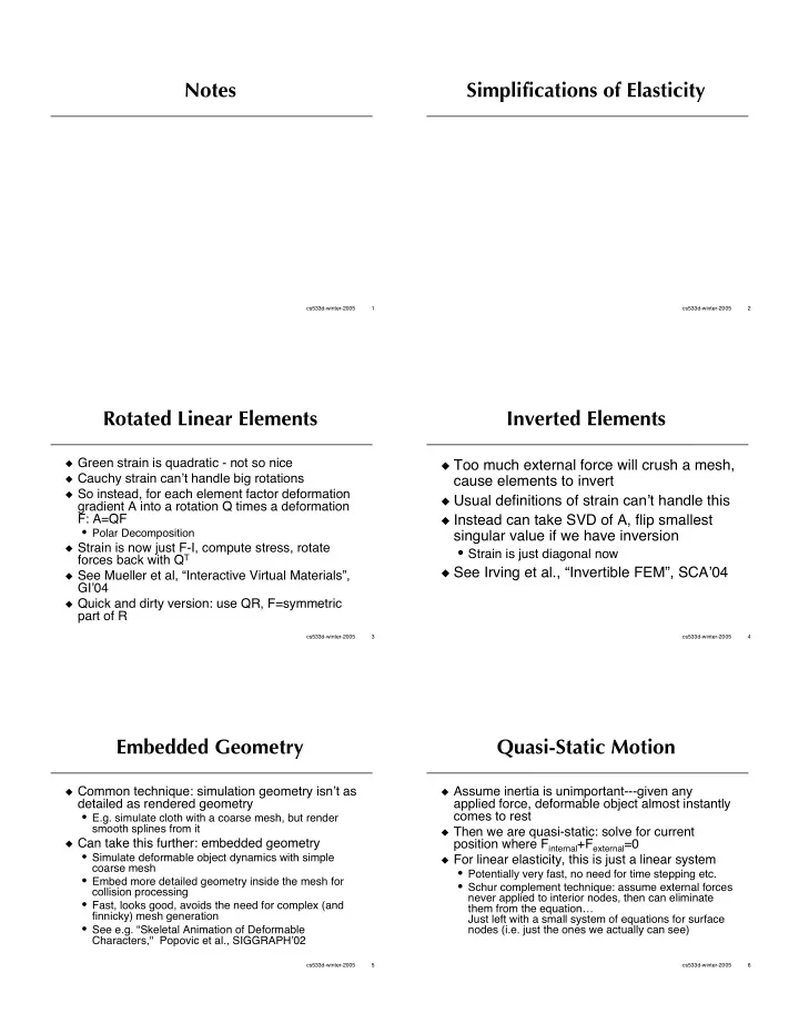
Notes Simplifications of Elasticity cs533d-winter-2005 1 cs533d-winter-2005 2 Rotated Linear Elements Inverted Elements � Green strain is quadratic - not so nice � Too much external force will crush a mesh, � Cauchy strain can’t handle big rotations cause elements to invert � So instead, for each element factor deformation � Usual definitions of strain can’t handle this gradient A into a rotation Q times a deformation F: A=QF � Instead can take SVD of A, flip smallest • Polar Decomposition singular value if we have inversion � Strain is now just F-I, compute stress, rotate • Strain is just diagonal now forces back with Q T � See Irving et al., “Invertible FEM”, SCA’04 � See Mueller et al, “Interactive Virtual Materials”, GI’04 � Quick and dirty version: use QR, F=symmetric part of R cs533d-winter-2005 3 cs533d-winter-2005 4 Embedded Geometry Quasi-Static Motion � Common technique: simulation geometry isn’t as � Assume inertia is unimportant---given any detailed as rendered geometry applied force, deformable object almost instantly comes to rest • E.g. simulate cloth with a coarse mesh, but render smooth splines from it � Then we are quasi-static: solve for current � Can take this further: embedded geometry position where F internal +F external =0 • Simulate deformable object dynamics with simple � For linear elasticity, this is just a linear system coarse mesh • Potentially very fast, no need for time stepping etc. • Embed more detailed geometry inside the mesh for • Schur complement technique: assume external forces collision processing never applied to interior nodes, then can eliminate • Fast, looks good, avoids the need for complex (and them from the equation… finnicky) mesh generation Just left with a small system of equations for surface • See e.g. “Skeletal Animation of Deformable nodes (i.e. just the ones we actually can see) Characters," Popovic et al., SIGGRAPH’02 cs533d-winter-2005 5 cs533d-winter-2005 6

Boundary Element Method Modal Dynamics � For quasi-static linear elasticity and a � See Pentland and Williams, “Good Vibrations”, homogeneous material, can set up PDE to SIGGRAPH’89 eliminate interior unknowns---before � Again assume linear elasticity discretization � Equation of motion is Ma+Dv+Kx=F external • Very accurate and efficient! � M, K, and D are constant matrices • Essentially the limit of the Schur complement • M is the mass matrix (often diagonal) approach… • K is the stiffness matrix � See James & Pai, “ArtDefo…”, SIGGRAPH’99 • D is the damping matrix: assume a multiple of K • For interactive rates, can actually do more: preinvert � This a large system of coupled ODE’s now BEM stiffness matrix � We can solve eigen problem to diagonalize and • Need to be smart about updating inverse when decouple into scalar ODE’s boundary conditions change… • M and K are symmetric, so no problems here - complete orthogonal basis of real eigenvectors cs533d-winter-2005 7 cs533d-winter-2005 8 Eigenstuff Decoupling into modes � Take y=U T x (so x=Uy) - decompose positions (and � Say U=(u 1 | u 2 | … | u 3n ) is a matrix with velocities, accelerations) into a sum of modes the columns the eigenvectors of M -1 K (also y = � M � 1 KUy � M � 1 DU ˙ y + M � 1 F ext U ˙ ˙ M -1 D) � Multiply by U T to decompose equations into modal • M -1 Ku i = � i u i and M -1 Du i = µ i u i components: y = � U T M � 1 KUy � U T M � 1 DU ˙ y + U T M � 1 F ext • Assume � i are increasing U T U ˙ ˙ • We know � 1 =…= � 6 =0 and µ 1 =…= µ 6 =0 y + U T M � 1 F ext ˙ y = � diag � i ˙ ( ) y � diag µ i ( ) ˙ (with u 1 , …, u 6 the rigid body modes) � So now we have 3n independent ODE’s • The rest are the deformation modes: the • If F ext is constant over the time step, can even write down exact formula for each larger that � i is, the smaller scale the mode is � Change equation of motion to this basis… cs533d-winter-2005 9 cs533d-winter-2005 10 Examining modes Throw out high frequencies � Mode i: � Only track a few low-frequency modes (5-10) i + u i � M � 1 F ext ˙ ˙ i = � � i y i � µ i ˙ y y � Time integration is blazingly fast! � Rigid body modes have zero eigenvalues, so just � Essentially reduced the degrees of freedom from depend on force thousands or millions down to 10 or so • Roughly speaking, rigid translations will take average of force, rigid rotations will take cross-product of force with positions • But keeping full geometry, just like embedded (torque) element approach • Better to handle these as rigid body… � Collision impulses need to be decomposed into � The large eigenvalues (large i) have small length scale, modes just like external forces oscillate (or damp) very fast • Visually irrelevant � Left with small eigenvalues being important cs533d-winter-2005 11 cs533d-winter-2005 12

Simplifying eigenproblem More savings � Low frequency modes not affected much by high � External forces (other than gravity, which frequency geometry is in the rigid body modes) rarely applied • And visually, difficult for observers to quantify if a mode is to interior, and we rarely see the interior actually accurate � So we can use a very coarse mesh to get the modes, or deformation even analytic solutions for a block of comparable mass � So just compute and store the boundary distribution particles � Or use a Rayleigh-Ritz approximation to the eigensystem (eigen-version of Galerkin FEM) • E.g. see James and Pai, “DyRT…”, • E.g. assume low frequency modes are made up of affine and SIGGRAPH’02 -- did this in graphics quadratic deformations hardware! • [Do FEM, get eigenvectors to combine them] cs533d-winter-2005 13 cs533d-winter-2005 14 Inelasticity: Plasticity & Fracture Plasticity & Fracture � If material deforms too much, becomes permanently deformed: plasticity • Yield condition: when permanent deformation starts happening (“if stress is large enough”) • Elastic strain: deformation that can disappear in the absence of applied force • Plastic strain: permanent deformation accumulated since initial state • Total strain: total deformation since initial state • Plastic flow: when yield condition is met, how elastic strain is converted into plastic strain � Fracture: if material deforms too much, breaks • Fracture condition: “if stress is large enough” cs533d-winter-2005 15 cs533d-winter-2005 16 For springs (1D) Fracturing meshes (1D) � Go back to Terzopoulos and Fleischer � Breaking springs leads to volume loss: material � Plasticity: change the rest length if the stress disappears (tension) is too high � Solutions: • Maybe different yielding for compression and tension • Break at the nodes instead (look at average tension • Work hardening: make the yield condition more around a node instead of on a spring) stringent as material plastically flows � Note: recompute mass of copied node • Creep: let rest length settle towards current length at • Cut the spring in half, insert new nodes a given rate � Note: could cause CFL problems… � Fracture: break the spring if the stress is too • Virtual node algorithm high � Embed fractured geometry, copy the spring (see Molino et al. • Without plasticity: “brittle” “A Virtual Node Algorithm…” SIGGRAPH’04) • With plasticity first: “ductile” cs533d-winter-2005 17 cs533d-winter-2005 18

Multi-Dimensional Plasticity Multi-Dimensional Yield criteria � Simplest model: total strain is sum of � Lots of complicated stuff happens when materials yield elastic and plastic parts: � = � e + � p • Metals: dislocations moving around � Stress only depends on elastic part • Polymers: molecules sliding against each other (so rest state includes plastic strain): • Etc. � = � ( � e ) � Difficult to characterize exactly when plasticity � If � is too big, we yield, and transfer some (yielding) starts of � e into � p so that � is acceptably small • Work hardening etc. mean it changes all the time too � Approximations needed • Big two: Tresca and Von Mises cs533d-winter-2005 19 cs533d-winter-2005 20 Yielding Tresca yield criterion � First note that shear stress is the important � This is the simplest description: • Change basis to diagonalize � quantity • Look at normal stresses (i.e. the eigenvalues of � ) • Materials (almost) never can permanently • No yield if � max - � min � � Y change their volume � Tends to be conservative (rarely predicts • Plasticity should ignore volume-changing yielding when it shouldn’t happen) stress � But, not so accurate for some stress states � So make sure that if we add kI to � it • Doesn’t depend on middle normal stress at all doesn’t change yield condition � Big problem (mathematically): not smooth cs533d-winter-2005 21 cs533d-winter-2005 22 Von Mises yield criterion � If the stress has been diagonalized: 1 2 + � 2 � � 3 2 + � 3 � � 1 2 � � Y ( ) ( ) ( ) � 1 � � 2 2 � More generally: 2 � 1 2 � � Y ( ) 3 � F 3 Tr � 2 � This is the same thing as the Frobenius norm of the deviatoric part of stress • i.e. after subtracting off volume-changing part: ( ) I F � � Y 3 2 � � 1 3 Tr � cs533d-winter-2005 23