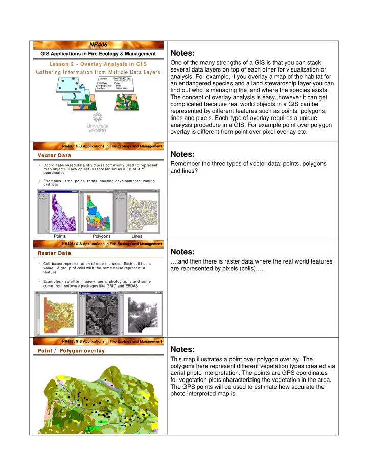
Notes: GIS Applications in Fire Ecology & Management One of the - PDF document

NR406 Notes: GIS Applications in Fire Ecology & Management One of the many strengths of a GIS is that you can stack Lesson 2 - Overlay Analysis in GI S several data layers on top of each other for visualization or Gathering Information from Multiple Data Layers analysis. For example, if you overlay a map of the habitat for an endangered species and a land stewardship layer you can find out who is managing the land where the species exists. The concept of overlay analysis is easy, however it can get complicated because real world objects in a GIS can be represented by different features such as points, polygons, lines and pixels. Each type of overlay requires a unique analysis procedure in a GIS. For example point over polygon overlay is different from point over pixel overlay etc. NR406: GIS Applications in Fire Ecology and Management Notes: Vector Data Vector Data Remember the three types of vector data: points, polygons • Coordinate-based data structures comm only used to represent map objects. Each object is represented as a list of X,Y and lines? coordinates • Examples - tree, poles, roads, housing developments, zoning districts Points Polygons Lines NR406: GIS Applications in Fire Ecology and Management Notes: Raster Data Raster Data ….and then there is raster data where the real world features • Cell-based representation of map features. Each cell has a are represented by pixels (cells)…. value. A group of cells with the same value represent a feature. • Examples - satellite imagery, aerial photography and some come from software packages like GRID and ERDAS. NR406: GIS Applications in Fire Ecology and Management Notes: Point / Polygon overlay Point / Polygon overlay This map illustrates a point over polygon overlay. The polygons here represent different vegetation types created via aerial photo interpretation. The points are GPS coordinates for vegetation plots characterizing the vegetation in the area. The GPS points will be used to estimate how accurate the photo interpreted map is.

NR406: GIS Applications in Fire Ecology and Management Notes: Point / GRI D overlay Point / GRI D overlay This is a similar map where the vegetation layer was created via image analysis of a satellite image resulting in a raster dataset (grid) where all green pixels represent vegetation type 1, the brown pixels vegetation type 2 etc. Again, the orange points are GPS locations for ground control points. NR406: GIS Applications in Fire Ecology and Management Notes: “Piercing Needle” Approach “Piercing Needle” Approach Two overlay analysis principles will be described here: 1 – the • Multiple layers of data are in piercing needle approach 2 – the cookie cutter approach. relative position with one another - inserting a "digital pin" through Both methods involves extracting data from multiple GIS data the stack of overlayed data. layers at locations of interest. In the ‘piercing needle approach’ information from one or more data layers are • This allows questions to be extracted at one single point (point – polygon overlay). For answered concerning everything occurring at a particular location. example, you may want to know the habitat type and canopy cover at bird nest locations. In this case the bird nests are • This view of the world limits represented by a point layer and the habitat type, elevation focus to a particular point and and canopy cover is represented by individual polygon data precludes wide-area landscape layers. The result of such an analysis will be a table that analysis. contains the habitat type and canopy cover for each bird nest location in your dataset. NR406: GIS Applications in Fire Ecology and Management Notes: GI S Overlay Analysis - Points GI S Overlay Analysis - Points This table gives you information on what tool in ArcGIS (or Overlay type ArcView 3x ArcGIS 9x ArcInfo ArcView 3.x or ArcInfo) you can use to create a point to Workstation polygon or point to grid overlay. For example in a Point to Polygon Geoprocessing Join and Relates: Arc: identity Wizard – Spatial Join – Join data point/polygon overlay, to find the polygon characteristics of Join based on spatial location the locations where the points are located, use the Join and Relates features. In Exercise 2 which is part of this lesson you Point to Grid Spatial Analyst: Spatial Analyst: GRID: sample Analysis – Tabulate Raster Calculator will perform these different kinds of overlay analyses. Areas or Toolbox – Spatial Script: Analyst Tools- samplegrids.ave Extraction- Extract by Points or Sample NR406: GIS Applications in Fire Ecology and Management Notes: Polygon Overlays – on polygons or grids Polygon Overlays – on polygons or grids Sometimes we want to overlay a polygon layer over another polygon layer or a raster. In the map above the polygons outlined in black represent fire perimeters and the raster map What covertypes represents different cover types. An overlay analysis can here burned in the Selway- tell you the cover types within the fire perimeters. Bitterrot Wilderness in year 2000? Fire perimeters 2000