Notes Adams-Bashforth Adams-Bashforth family are examples of Notes - - PDF document

SLIDE 1

1 cs542g-term1-2007

Notes

Notes for last part of Oct 11 and all of Oct 12

lecture online now

Another extra class this Friday 1-2pm

2 cs542g-term1-2007

Adams-Bashforth

Adams-Bashforth family are examples of

linear multistep methods

• Linear: the new y is a linear combination of ys and fs
• Multistep: the new y depends on several old values

Efficient

• Can get high accuracy with just one evaluation of f

per time step

• Can even switch order/accuracy as you go

Reasonably stable

• AB3 and higher include some of the imaginary axis

Rephrased as a “multivalue method”, can easily

accommodate variable time steps…

3 cs542g-term1-2007

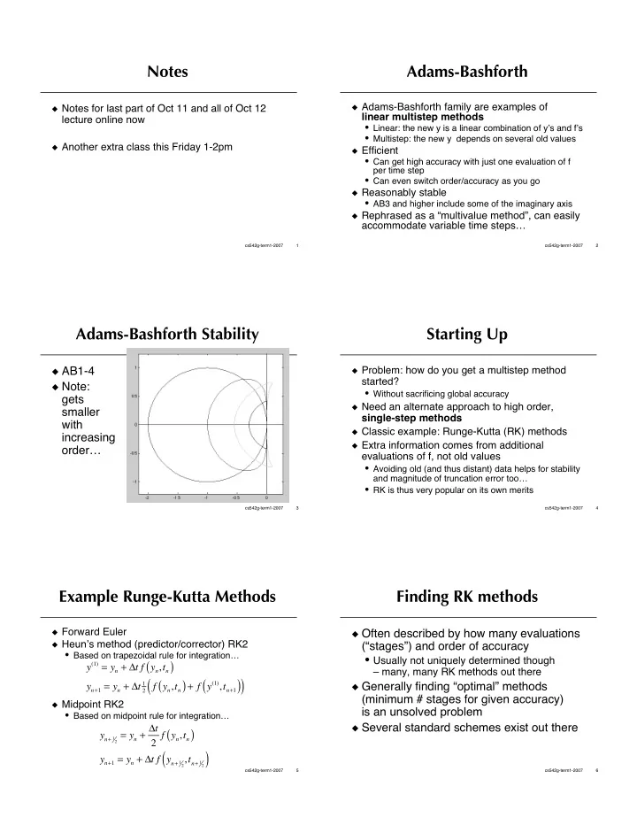
Adams-Bashforth Stability

AB1-4 Note:

gets smaller with increasing

• rder…

4 cs542g-term1-2007

Starting Up

Problem: how do you get a multistep method

started?

• Without sacrificing global accuracy

Need an alternate approach to high order,

single-step methods

Classic example: Runge-Kutta (RK) methods Extra information comes from additional

evaluations of f, not old values

• Avoiding old (and thus distant) data helps for stability

and magnitude of truncation error too…

• RK is thus very popular on its own merits

5 cs542g-term1-2007

Example Runge-Kutta Methods

Forward Euler Heuns method (predictor/corrector) RK2

• Based on trapezoidal rule for integration…

Midpoint RK2

• Based on midpoint rule for integration…

y(1) = yn + t f yn,tn

( )

yn+1 = yn + t 1

2 f yn,tn

( ) + f y(1),tn+1

( )

( )

yn+ 12 = yn + t 2 f yn,tn

( )

yn+1 = yn + t f yn+ 12,tn+ 12

( )

6 cs542g-term1-2007

Finding RK methods

Often described by how many evaluations

(“stages”) and order of accuracy

• Usually not uniquely determined though

–many, many RK methods out there

Generally finding “optimal” methods

(minimum # stages for given accuracy) is an unsolved problem

Several standard schemes exist out there

SLIDE 2

7 cs542g-term1-2007

Classic RK4

Probably the most widely used higher

• rder time integration scheme

k1 = t f yn,tn

( )

k2 = t f yn + 1

2 k1,tn+ 12

( )

k3 = t f yn + 1

2 k2,tn+ 12

( )

k4 = t f yn + k3,tn+1

( )

yn+1 = yn + 1 6 k1 + 2k2 + 2k3 + k4

( )

8 cs542g-term1-2007

Runge-Kutta Stability

Forward Euler 2-stage RK2 3-stage RK3 4-stage RK4 Can trade

accuracy for stability…

9 cs542g-term1-2007

Adaptive time steps

General idea: take large time steps where

solution is smooth

• Truncation error is

Example approach:

• Use pth and p+1st order integrators
• Difference estimates error of pth order scheme
• Modify t for next time step to attempt to keep error

per unit time constant

• N.B.: use p+1st order answer to go forward…

Runge-Kutta-Fehlberg (RKF) pairs:

can sometimes reuse much of computation of pth method to get p+1st method O t p py t p

• 10

cs542g-term1-2007

Looking at error

Heuristic error control isnt guaranteed! Usual validation approaches:

• Test your method on a known exact solution
• Test your method against real experimental

data (modeling error also included)

• Run solver multiple times, with smaller and

smaller time steps

Plot error against t Look at ratio of error when t halved

11 cs542g-term1-2007

Stiffness

Things may go wrong however! Simple example: Forward Euler stability restriction:

always need t < 0.002

First order accuracy:

for t>0.05, can use gigantic t

Problem is stiffness: stability of method requires

much smaller time step than accuracy demands

So far we cant efficiently solve stiff problems

dy dt = 11000 y t

( ),

y 0

( ) = 1

12 cs542g-term1-2007

Stiffness analyzed

Usually results from hugely different

time-scales in the problem

Linear example: The “fast” mode may be transient–quickly

decays to zero–so the “slow” mode determines truncation error

But the “fast” mode determines stability

time step restriction

dy dt = 100 0.01

• y

SLIDE 3

13 cs542g-term1-2007

Reversing time

Consider with positive real part Unstable when going forwards in time

(and FE etc. are similarly unstable, particularly for big time steps)

Now, reverse time

• Exponential growth, in reverse, is stable

exponential decay

• Reversed methods are stable!

Equivalent to regular time, with negative

real part

14 cs542g-term1-2007

Backwards Euler

Backwards Euler: reverse version of FE This is an implicit method:

new y defined implicitly (appears on both sides)

Methods from previous slides are all explicit:

new y explicitly computed from known values

Going implicit is the key to handling stiffness

yn+1 = yn + t f yn+1,tn+1

( )

15 cs542g-term1-2007

Other implicit methods

Backwards Euler is over-stable: A-stable: region of stability includes left

half-plane (stable when exact solution is)

Implicit mid-point Trapezoidal rule

1 t > 1 yn+1 = yn + t f

1 2 yn + 1 2 yn+1,tn+ 12

( )

yn+1 = yn + t

1 2 f yn,tn

( ) + 1

2 f yn+1,tn+1

( )

• 16

cs542g-term1-2007

Even more

Implicit multistep methods:

Adams(-Bashforth)-Moulton Backwards Differentiation Formula (BDF)

Implicit Runge-Kutta

• Might need to solve for multiple intermediate

values simultaneously…