Normal Distributions MATH 107: Finite Mathematics University of - PDF document

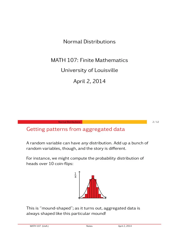
Normal Distributions MATH 107: Finite Mathematics University of Louisville April 2, 2014 Normal Distributions 2 / 12 Getting patterns from aggregated data A random variable can have any distribution. Add up a bunch of random variables, though, and the story is di ff erent. For instance, we might compute the probability distribution of heads over 10 coin-flips: 1 4 This is “mound-shaped”; as it turns out, aggregated data is always shaped like this particular mound! MATH 107 (UofL) Notes April 2, 2014

Normal Distributions 3 / 12 The normal distribution σ σ µ This shape, to which all aggregated data tends, is called the “normal” or “Gaussian” distribution. It has the awful equation: e −( x − µ ) 2 / 2 σ 2 √ 2 π σ π here is the beloved constant (about 3.141592); σ and µ describe the positioning of the curve. µ is the mean : the center and highest point of the curve. σ is the standard deviation , which quantifies spread. MATH 107 (UofL) Notes April 2, 2014 Normal Distributions 4 / 12 Normally distributed features Many everyday features are normally distributed. Some normally distributed population features ▸ Adult height in women: µ = 64 inches, σ = 3 inches. ▸ IQ: µ = 100, σ = 15. Based on these, if we understand normal distributions, we can work out probabilities in the population! MATH 107 (UofL) Notes April 2, 2014

Normal Distributions 5 / 12 Finding population stats A simple statistical question What percentage of women are more than 60 inches tall? 3 3 60 64 This curve describes the distribution of women’s heights. We want to know what proportion of the population is in the shaded area. MATH 107 (UofL) Notes April 2, 2014 Normal Distributions 6 / 12 Standardizing curves 3 3 1 1 � ⇒ 60 64 − 4 3 Having to know a lot about every normal curve would be di ffi cult. Instead, we look at a standard normal curve with µ = 0 and σ = 1. We map 60 on the old curve to a position on the new curve called a z -value: z = x − µ σ So now we want to know what’s to the right of − 4 3 on the standard normal curve . MATH 107 (UofL) Notes April 2, 2014

Normal Distributions 7 / 12 The bad news − 4 3 There is no easy way to determine this area! There are complicated computations which have been done in advance. Table 1 in Appendix C has a list of these computations. MATH 107 (UofL) Notes April 2, 2014 Normal Distributions 8 / 12 Using a table − 4 3 We’re interested in what happens at − 4 3 ≈ − 1 . 33. ⋯ .03 ⋯ ⋮ ⋮ ⋮ ⋮ We look up 1.33 in our table: ⋯ ⋯ 1.3 0.4082 ⋮ ⋮ ⋮ ⋮ That’s the area between 0 and 1 . 33 on the graph. 4 3 This is not quite what we want, but it’s close; we add 1 MATH 107 (UofL) Notes April 2, 2014 2 to get the real thing: 0 . 4082 + 0 . 5 = 90 . 82 % .

Normal Distributions 9 / 12 General approach To find the probability of a given range in a normal curve: ▸ Translate both ends of the range to z -values: z = x − µ σ . ▸ Look up the absolute value of each end in a table, taking 1 2 as the answer when an end is open. ▸ Reverse the sign on either end which has negative z -value. ▸ Subtract the two table-results. MATH 107 (UofL) Notes April 2, 2014 Normal Distributions 10 / 12 Examples Characterization of IQ IQs are normally distributed around 100 with a standard deviation of 15. How likely is an IQ of between 110 and 130? x 1 = 110 → z 1 = 110 − 100 ≈ 0 . 66 → p 1 = 0 . 2454 15 x 2 = 130 → z 2 = 130 − 100 = 2 . 00 → p 2 → 0 . 4772 15 so the likelihood is 0 . 4772 − 0 . 2454 = 23 . 18 % . MATH 107 (UofL) Notes April 2, 2014

Normal Distributions 11 / 12 Examples Characterization of IQ IQs are normally distributed around 100 with a standard deviation of 15. How likely is an IQ of less than 120? x 1 = −∞ → p 1 = − 0 . 5 x 2 = 150 → z 2 = 120 − 100 ≈ 1 . 33 → p 2 → 0 . 4082 15 so the likelihood is 0 . 4082 −(− 0 . 5 ) = 90 . 82 % . MATH 107 (UofL) Notes April 2, 2014 Normal Distributions 12 / 12 Yet Another Example Manufacturing Your factory produces washers with an interior diameter of 15mm; due to manufacturing variance the washers actually have normally distributed diameter with standard deviation of 0.14mm. For high-precision applications, these washers need to have interior diameter between 14 . 9mm and 15 . 05mm. What proportion of our washers are suitable for high-precision applications? x 1 = 14 . 90 → z 1 = 14 . 90 − 15 ≈ − 0 . 71 → p 1 = − 0 . 2611 0 . 14 x 2 = 15 . 05 → z 2 = 15 . 05 − 15 ≈ 0 . 36 → p 2 → 0 . 1406 0 . 14 so 0 . 1406 −(− 0 . 2611 ) = 40 . 17 % of our washers will be su ffi ciently precise. MATH 107 (UofL) Notes April 2, 2014