Bayes Formula MATH 107: Finite Mathematics University of Louisville - PDF document

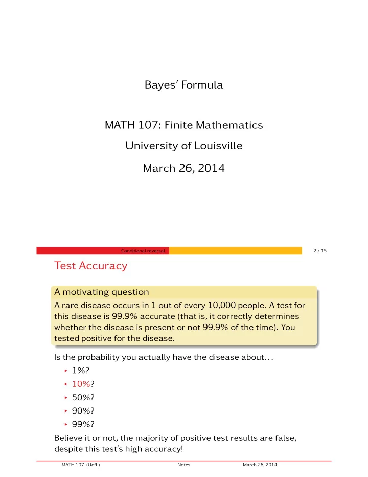
Bayes’ Formula MATH 107: Finite Mathematics University of Louisville March 26, 2014 Conditional reversal 2 / 15 Test Accuracy A motivating question A rare disease occurs in 1 out of every 10,000 people. A test for this disease is 99.9% accurate (that is, it correctly determines whether the disease is present or not 99.9% of the time). You tested positive for the disease. Is the probability you actually have the disease about... ▸ 1%? ▸ 10%? ▸ 50%? ▸ 90%? ▸ 99%? Believe it or not, the majority of positive test results are false, despite this test’s high accuracy! MATH 107 (UofL) Notes March 26, 2014

Conditional reversal 3 / 15 Justification of that result There are four possible classifications for any person: they could have the disease or not, and could test positive or negative. Let’s look at how we would expect 10,000,000 people to be classified: Test positive Test negative Total Have disease 999 1 1,000 No disease 9,999 9,989,001 9,999,000 Total 10,998 9,989,002 10,000,000 1 of every 10,000 people has the disease. In each category, 1 of every 1,000 people gets the wrong test result. We know we’re one of the 10,998 people who test positive; but only 999 of those have the disease, so our chances of having the disease are: 999 10998 ≈ 9 % MATH 107 (UofL) Notes March 26, 2014 Conditional reversal 4 / 15 What we’re doing here: as trees We could have phrased the original setup in the problem as a tree: 0 . 999 Positive test Disease 0 . 0001 Negative test 0 . 001 Start 0 . 001 Positive test 0 . 9999 No disease Negative test 0 . 999 And then the problem raised was reversing the tree: ? Disease Positive test ? ? No disease Start ? Disease ? Negative test ? No disease MATH 107 (UofL) Notes March 26, 2014

Conditional reversal 5 / 15 What we’re doing here: as events We could identify the disease as event D , and a positive test as T . The scenario told us that P ( D ) = 0 . 0001, and that P ( T ∣ D ) = P ( T ′ ∣ D ′ ) = 0 . 999. The question at the end of the scenario was to evaluate P ( D ∣ T ) . Thus, in a nutshell, what we want to do is reverse conditional probabilities which we know. MATH 107 (UofL) Notes March 26, 2014 Bayes’ Formula 6 / 15 Deriving a formula Suppose we know P ( A ) , P ( B ∣ A ) , and P ( B ∣ A ′ ) . How do we find P ( A ∣ B ) ? P ( A ∣ B ) = P ( A ∩ B ) P ( B ) = P ( B ∣ A ) P ( A ) P ( B ) P ( B ∣ A ) P ( A ) = P ( A ∩ B )+ P ( A ′ ∩ B ) P ( B ∣ A ) P ( A ) = P ( B ∣ A ) P ( A )+ P ( B ∣ A ′ ) P ( A ′ ) P ( B ∣ A ) P ( A ) = P ( B ∣ A ) P ( A )+ P ( B ∣ A ′ )( 1 − P ( A )) This is one of several variations on what is known as Bayes’ formula . MATH 107 (UofL) Notes March 26, 2014

Bayes’ Formula 7 / 15 Using Bayes’ formula P ( B ∣ A ) P ( A ) P ( A ∣ B ) = P ( B ∣ A ) P ( A )+ P ( B ∣ A ′ )( 1 − P ( A )) In our disease example, the disease (event A ) had probability 0 . 0001, while the test (event B ) occurred with conditional probabilities P ( B ∣ A ′ ) = 0 . 001 and P ( B ∣ A ) = 0 . 999, so: 0 . 999 × 0 . 0001 P ( A ∣ B ) = 0 . 999 × 0 . 0001 + 0 . 001 × 0 . 9999 ≈ 0 . 0908 as we had previously worked out. MATH 107 (UofL) Notes March 26, 2014 Bayes’ Formula 8 / 15 Detecting a fake An unfair coin problem We have two coins, one of which is fair and the other of which lands heads-up 75% of the time, but we don’t know which is which. We pick a random coin and flip it eight times and get the results HHHHHTHT. This looks like it’s the unfair one, but how certain can we be? We have two events: A is the event that the chosen coin is in fact the unfair one, and B would be the event that 8 coin flips come out the way ours did. What we want to find is P ( A ∣ B ) . We know: 6 2 8 P ( A ) = 1 2 ; P ( B ∣ A ) = ( 3 ( 1 ; P ( B ∣ A ′ ) = ( 1 4 ) 4 ) 2 ) MATH 107 (UofL) Notes March 26, 2014

Bayes’ Formula 9 / 15 Detecting a fake, continued P ( A ) = 1 2 ; P ( B ∣ A ) = 729 2 12 ; P ( B ∣ A ′ ) = 1 2 6 We apply Bayes’ formula: P ( B ∣ A ) P ( A ) P ( A ∣ B ) = P ( B ∣ A ) P ( A )+ P ( B ∣ A ′ )( 1 − P ( A )) 2 12 × 1 729 = 2 2 12 × 1 2 + 1 2 6 × 1 729 2 = 729 793 ≈ 92 % which is a good but not ironclad certainty that we have the right choice. MATH 107 (UofL) Notes March 26, 2014 Bayes’ Formula 10 / 15 Another variation on Bayes’ theorem Sometimes instead of having a single prior result we want to find, we might have one of several mutually exclusive possibilities. We might have mutually exclusive events A 1 , A 2 ,..., A n with total probability 1 and an event B , and want to find P ( A 1 ∣ B ) from all the P ( A i ) and P ( B ∣ A i ) : P ( A 1 ∣ B ) = P ( A 1 ∩ B ) P ( B ) = P ( B ∣ A 1 ) P ( A 1 ) P ( B ) P ( B ∣ A 1 ) P ( A 1 ) = P ( A 1 ∩ B )+ P ( A 2 ∩ B )+⋯+ P ( A n ∩ B ) P ( B ∣ A 1 ) P ( A 1 ) = P ( B ∣ A 1 ) P ( A 1 )+ P ( B ∣ A 2 ) P ( A 2 )+⋯+ P ( B ∣ A n ) P ( A n ) MATH 107 (UofL) Notes March 26, 2014

Bayes’ Formula 11 / 15 A multiple-possibility scenario Two fake coins! We now happen to have a collection of three coins; one fair, one of which lands heads-up 3 4 of the time, and one of which lands tails-up 3 4 of the time. We pick one at random, flip it 7 times, and get the result TTHHHTH. What is the chance we chose the fair coin? Let A 1 be the event of picking the fair coin, A 2 the event of picking the heads-biased coin, A 3 the event of picking the tail-biased coin, and B the event of flipping our chosen coin to get TTHHHTH. We want to know P ( A 1 ∣ B ) .Clearly, each P ( A i ) = 1 3 , and: 7 4 3 3 4 P ( B ∣ A 1 ) = ( 1 ; P ( B ∣ A 2 ) = ( 3 ( 1 ; P ( B ∣ A 3 ) = ( 3 ( 1 2 ) 4 ) 4 ) 4 ) 4 ) . MATH 107 (UofL) Notes March 26, 2014 Bayes’ Formula 12 / 15 A multiple-possibility scenario, cont’d P ( A 1 ) = P ( A 2 ) = P ( A 3 ) = 1 3 ; P ( B ∣ A 1 ) = 1 2 7 ; P ( B ∣ A 2 ) = 81 4 7 ; P ( B ∣ A 3 ) = 27 4 7 We apply Bayes’ formula: P ( B ∣ A 1 ) P ( A 1 ) P ( A 1 ∣ B ) = P ( B ∣ A 1 ) P ( A 1 )+ P ( B ∣ A 2 ) P ( A 2 )+ P ( B ∣ A 3 ) P ( A 3 ) 2 7 × 1 1 = 3 2 7 × 1 3 + 81 4 7 × 1 3 + 27 4 7 × 1 1 3 = 128 236 ≈ 54 % which is better than a blind guess (right 33% of the time), but not by much! MATH 107 (UofL) Notes March 26, 2014

Bayes’ Formula 13 / 15 Another unequal-probability scenario Two unfair coins...and lots of fair ones! Our heads-up (75%) and tails-up (75%) coins are mixed in with eight normal coins. We pick one at random, flip it 6 times, and get all heads. What are the probabilities we got the heads-biased coin? The tails-biased coin? A fair coin? Let A 1 be the event of picking a fair coin, A 2 the event of picking the heads-biased coin, A 3 the event of picking the tail-biased coin, and B the event of flipping six heads. We’re interested in the three conditional probabilities P ( A i ∣ B ) . P ( A 1 ) = 0 . 8 ; P ( A 2 ) = P ( A 3 ) = 0 . 1 2 6 ; P ( B ∣ A 2 ) = 3 6 P ( B ∣ A 1 ) = 1 4 6 ; P ( B ∣ A 3 ) = 1 4 6 MATH 107 (UofL) Notes March 26, 2014 Bayes’ Formula 14 / 15 Another unequal-probability scenario, cont’d Applying Bayes’ formula: P ( B ∣ A 1 ) P ( A 1 ) P ( A 1 ∣ B ) = P ( B ∣ A 1 ) P ( A 1 )+ P ( B ∣ A 2 ) P ( A 2 )+ P ( B ∣ A 3 ) P ( A 3 ) 2 6 × 0 . 8 1 = 256 = 621 ≈ 41 % 2 6 × 0 . 8 + 729 4 6 × 0 . 1 + 1 4 6 × 0 . 1 1 P ( B ∣ A 2 ) P ( A 2 ) P ( A 2 ∣ B ) = P ( B ∣ A 1 ) P ( A 1 )+ P ( B ∣ A 2 ) P ( A 2 )+ P ( B ∣ A 3 ) P ( A 3 ) 4 6 × 0 . 1 729 = 729 = 1242 ≈ 59 % 2 6 × 0 . 8 + 729 4 6 × 0 . 1 + 1 4 6 × 0 . 1 1 P ( B ∣ A 3 ) P ( A 3 ) P ( A 3 ∣ B ) = P ( B ∣ A 1 ) P ( A 1 )+ P ( B ∣ A 2 ) P ( A 2 )+ P ( B ∣ A 3 ) P ( A 3 ) 4 6 × 0 . 1 1 1 = = 1242 ≈ 0 . 08 % 2 6 × 0 . 8 + 729 4 6 × 0 . 1 + 1 4 6 × 0 . 1 1 MATH 107 (UofL) Notes March 26, 2014

Bayes’ Formula 15 / 15 Where we use this In many problems, the real-world state is not yet known, and the test is all we have . Even the probabilities associated with the real-world state are often unknown! In practice, we often assume some simple probability distribution (called the prior probability ) for the real-world state, and use Bayes’ formula to figure out a distribution which better fits the evidence (called the posterior probability ). By using the posterior of one experiment to determine the prior of another, we can get a very accurate idea of the “true” underlying probabilities! This technique is known as Bayesian statistics . MATH 107 (UofL) Notes March 26, 2014