Nonequilibrium and statistical ensembles Statistical properties of - PowerPoint PPT Presentation

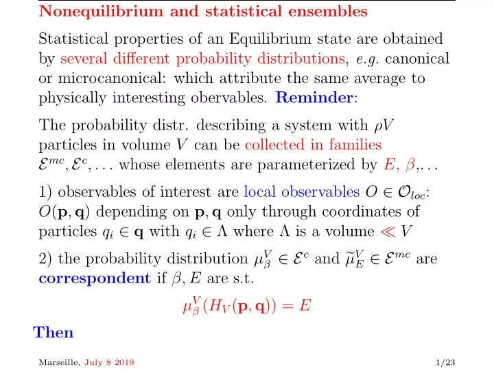
Nonequilibrium and statistical ensembles Statistical properties of an Equilibrium state are obtained by several different probability distributions, e.g. canonical or microcanonical: which attribute the same average to physically interesting obervables. Reminder : The probability distr. describing a system with ρV particles in volume V can be collected in families E mc , E c , . . . whose elements are parameterized by E , β ,. . . 1) observables of interest are local observables O ∈ O loc : O ( p , q ) depending on p , q only through coordinates of particles q i ∈ q with q i ∈ Λ where Λ is a volume ≪ V β ∈ E c and � E ∈ E mc are 2) the probability distribution µ V µ V correspondent if β, E are s.t. µ V β ( H V ( p , q )) = E Then Marseille, July 8 2019 1/23

V →∞ µ V µ V lim β ( O ) = lim V →∞ � E ( O ) and µ ’s are equivalent in the thermodynamic limit. In case of phase transitions extra labels γ, � γ are added to identify the extremal distributions and it is possible to establish a correspondence between the extra labels γ ← → � γ so that the equivalence can be equally formulated. Is it possible a similar description of the stationary states of nonequilibrium systems? Think an evolution eq. of u on a “phase space” M depending on a parameter R : u = f R ( u ) ˙ Typically eq. will be difficult and even existence-1-qness will be open problems. Marseille, July 8 2019 2/23

As an example consider infinitely many hard spheres of given density or a forced incompressible 3D NS fluid with periodic b.c.: at best only not constructive“weak solutions”. ⇒ the eq. will have to be regularized in f V R ( u ) where V is a regularization parameter. E.g. (1) in SM V is typically the container size: and the problem becomes finding the observables whose averages have a limit as V → ∞ : Physical observables. Such observables u → O ( u ) in SM are those only depending on points of u in region K ≪ V , “local observables”. (2) For the NS equation the regularization parameter could be a “UV cut-off” N . And it is natural to consider as physical observables the u → O ( u ) which only depend on the Fourier’s components k of u with | k | < K ≪ N . Marseille, July 8 2019 3/23

Once the class of physical observables is restricted, it is to be expected (?) that several equations of motion could describe the stationary states of the same system. E.g. the h.c. system can be described by the Hamilton eq.s but also by the isothermal equations p = − ∂ q V ( q ) − α ( p , q ) p q = p , ˙ ˙ where α ( p , q ) is a multiplier which imposes T ( p ) = const . Stationary states of the two equations are parameterized by energy E or by kinetic energy T ; stationary states will be µ mc,V = δ ( H ( p , q ) − E ) d p d q or, respectively : E β 0 = β (1 − 1 µ c,V = e − β 0 V ( q ) δ ( T ( p ) − Nβ − 1 ) d p d q , 3 N ) β Equivalent if µ c,V β ( H ) = E : lim V →∞ µ c,V β ( O ) = lim V →∞ µ mc,V ( O ). E Marseille, July 8 2019 4/23

Interesting cases arise when the system is described by equations which obey a symmetry but they are phenomenologically described by non symmetric equations (cases of spontaneously broken symmetry). Consider, as a typical case, the Navier-Stokes equation: in the case of the above incompressible fluid they can be regarded as Euler equations subject to a thermostat absorbing the heat due to the viscosity: which turns the equations into time-reversal breaking ones. A paradigmatic case is a fluid in a periodic container 2/3-Dim., incompressible, at fixed forcing F (smooth, e.g. with only one Forurier component non zero and � F � 2 = 1), kept at const. temp. by a thermostat. to dissipate heat via the force due to viscosity ν = 1 R (consistently with incompressibility). Marseille, July 8 2019 5/23

u · ∂ ) u α − ∂ α p + 1 u α = − ( � NS irr : ˙ R ∆ u α + F α , ∂ α u α = 0 u ( x ) = � i k ⊥ | k | e i k · x , Velocity: � 0 u k u k = u − k (NS-2D) k � = � � u k = � 1 · k 2 )( k 2 2 − k 2 ( k ⊥ 1 ) u k 1 u k 2 − ν k 2 u k + f k NS 2 ,irr : ˙ k 1 + k 2 = k 2 | k 1 || k 2 || k | Imagine to truncate eq. supposing | k j | ≤ N . Cut-off UV , N , is temporarily fixed ( BUT interest is on N → ∞ ). NS 2D → ODE in a phase space M N with 4 N ( N + 1) dimen. (In 3D O (8 N 3 )). Exist. & 1-ness trivial D = 2 , 3. BUT Iu α = − u α implies IS irr � = S irr − t I , ⇒ : irreversibility. t Given init. data u , evolution t → S irr t u generates a steady state ( i.e. a SRB probability distr.) µ irr,N on M N . R Unique aside a volume 0 of u ’s, for simplicity [ Not so at small R : “NS gauge symmetry” exists. ?? ] Marseille, July 8 2019 6/23

[1, 2, 3]. As R varies the steady distr. µ irr,N ( du ) form a R collection E irr,N : to be named A statistical ensemble of stationary nonequilibrium distrib. for NS irr . And average energy E R , average dissipation En R , Lyapunov spectra (local and global) ... will be defined, e.g. : � � M N µ irr,N M N µ irr,N ( du ) || u || 2 ( du ) || k u || 2 E R = 2 , En R = 2 R R Consider new equation, NS rev : � ( k ⊥ 1 · k 2 )( k 2 2 − k 2 1 ) u k 1 u k 2 − α ( u ) k 2 u k + f k u k = ˙ 2 | k 1 || k 2 || k | k 1 + k 2 = k with α s. t. D ( u ) = || k u || 2 2 = En (the enstrophy)is exact const of motion on u → S rev u .: t � k k 2 F − k u k ⇒ α ( u ) = � e . g . D = 2 k k 4 | u k | 2 Marseille, July 8 2019 7/23

New eq. is reversible: IS rev u = S rev − t Iu (as α is odd). t α is “a reversible viscosity”; (if D = 3 α is ∼ different) Rev. eq. can be considered as model of empirical “thermostat” acting on the fluid and should ( ? ) have same effect of empirical constant friction. NS rev generates a family of steady states E rev,N on M N : µ rev,N parameterized by constant value of enstrophy En . En α ( u ) in NS rev will wildly fluctuate at large R ( i.e. small viscosity ν ) thus “ self averaging ” to a const. value ν “homogenizing” the eq. into NS irr with viscosity ν . � k f k u k Of course we could impose a multiplier α ′ ( u ) = k | k | 2 | u k | 2 : � it would fix energy E = � k | u k | 2 and obtain diff. rev. eq. Marseille, July 8 2019 8/23

The equivalence mechanism is suggested by analogy with Stat. Mech. (1) analog of “local observables”: functions O ( u ) which depend only on u k with | k | < K . “Locality in momentum” (2) analog of “Volume”: just the cut-off N confining the k (3) analog of the “state parameter”: the viscosity ν = 1 R (irrev. case) or the enstrophy En (rev. case) (or energy E ). Equivalence is conjectured at N = ∞ corresponding to the Thermodynamic limit V → ∞ , for all R . Averages of large scale observables will tend to the same ∈ E irr,N of NS irr and for values as N → ∞ for µ irr,N R = � ∈ E rev,N provided, D ( u ) def k k 2 | u k | 2 is s.t. µ rev,N En ( α ) = 1 µ irr,N µ rev,N ( D ) = En, or R En R Marseille, July 8 2019 9/23

Remark that multiplying the NS eq. by u k and sum on k : � 1 d | u k | 2 = − γ D ( u ) + W ( u ) , γ = ν or α ( u ) 2 dt k here the transport terms = 0, D = 2 , 3, D ( u ) = � k k 2 | u k | 2 = enstrophy and W = � k f k u − k = work per unit time of the external force. Hence time averaging 1 Rµ irr,N ( D ) = µ irr,N µ rev,N ( α ) En = µ rev,N ( W ) , ( W ) R R En En But W is local (as f is such) and, if the conjecture holds, has equal average under the equivalence condition: hence µ irr,N ( D ) = En implies the relation R R →∞ Rµ rev,N lim ( α ) = 1 En Marseille, July 8 2019 10/23

This becomes a first rather stringent test of the conjecture. Since the equivalence rests on the rapid fluctuations of α ( u ) a second idea is that if N is kept finite then, more generally, if O is a large scale observable it should be: µ irr,N ( O ) = µ rev,N µ irr,N ( D ) = En ( O )(1+ o (1 /R )) if R En R So a different idea arises. In many phenomenological and dissipative equations of the form ˙ x = f ( x ) − ν x + g the ν can be replaced by α ( x ) so that E = x 2 =const.= If for ν = 0 , g = � 0 the motion is strongly chaotic then x = f ( x ) − ν x + g , ˙ α ( x ) = g · x x = f ( x ) − α ( x ) x + g , ˙ x 2 Equivalence if ν → 0 between stationary µ irr and µ rev if ν E µ irr ν ( α ) = E What is special to NS to conj. that R → ∞ is not needed? Marseille, July 8 2019 11/23

It is its being a scaling limit of a microscopic equation whose evolution is certainly chaotic and reversible. Therefore NS is different from the many phenomenological and dissipative equations which are not directly related to fundamental equations. For the latter cases strong chaos is necessary if a friction parameter is changed into a fluctuating quantity. There are many examples of phenomenological equations (1) (highly) truncated NS equations ( N < ∞ fixed), [4], (2) NS with Ekman friction ( − ν� u instead of ν ∆ � u ), [5, 6], (3) Lorenz96 model, [7], (4) Shell model of turbulence, (GOY), [8] In such equations R → ∞ is necessary: and, for each of them, it has been tested in few cases. Marseille, July 8 2019 12/23

But it will be useful to pause to illustrate a few prelimnary simulations and checks. Unfortunately the simulations are in dimension 2 ( D = 3 is at the moment beyond the available (to me) computational tools) although present day available NS codes should be perfectly capable to perform detailed checks in rapid time. Marseille, July 8 2019 13/23