Friction, reversibility, fluctuations in nonequilibrium and chaotic - PowerPoint PPT Presentation

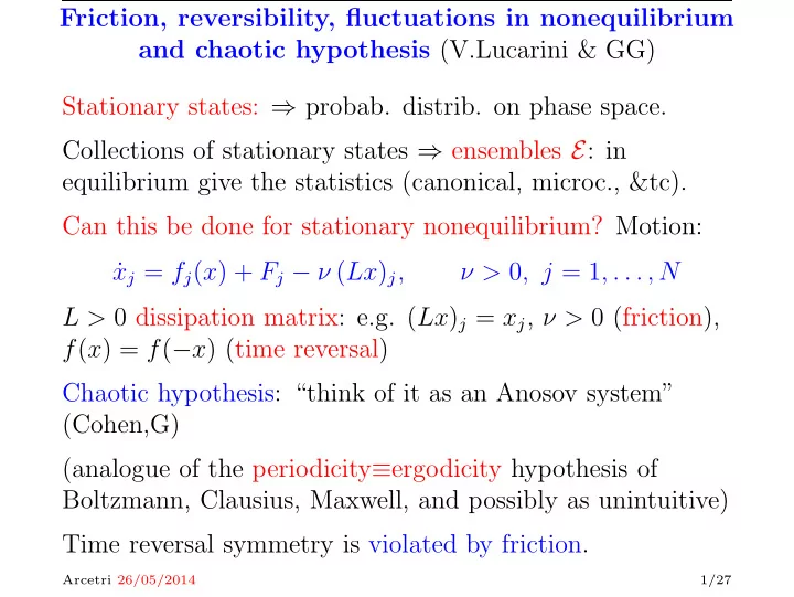
Friction, reversibility, fluctuations in nonequilibrium and chaotic hypothesis (V.Lucarini & GG) Stationary states: ⇒ probab. distrib. on phase space. Collections of stationary states ⇒ ensembles E : in equilibrium give the statistics (canonical, microc., &tc). Can this be done for stationary nonequilibrium? Motion: x j = f j ( x ) + F j − ν ( Lx ) j , ˙ ν > 0 , j = 1 , . . . , N L > 0 dissipation matrix: e.g. ( Lx ) j = x j , ν > 0 (friction), f ( x ) = f ( − x ) (time reversal) Chaotic hypothesis: “think of it as an Anosov system” (Cohen,G) (analogue of the periodicity ≡ ergodicity hypothesis of Boltzmann, Clausius, Maxwell, and possibly as unintuitive) Time reversal symmetry is violated by friction. Arcetri 26/05/2014 1/27

BUT it is a fundamental symmetry: ⇒ possible to restore? How? in which sense? Start from a special case: the Lorenz96 eq. (periodic b.c.) x j = x j − 1 ( x j +1 − x j − 2 ) + F − νx j , ˙ j = 0 , . . . , N − 1 Vary ν and let µ ν stationary distrib. Let E = � � x 2 j ˙ i � µ ν : this is “ensemble” (viscosity ensemble) Equivalent ensembles conjecture: replace ν by � i Fx i � α ( x ) = i x 2 i New Eq. has E ( x ) = � i x 2 i as exact constant of motion x j = x j − 1 ( x j +1 − x j − 2 ) + F − α ( x ) x j , ˙ and volume contracts by � ∂ j ( a ( x ) x j ) � τ p = τ − 1 σ ( x ) = ( N − 1) α ( x ) , σ ( x ( t )) dt/ � σ � 0 Arcetri 26/05/2014 2/27

Equivalent ensembles (conjecture): µ E label by E ⇒ � Stationary states � E (“energy ensemble”). µ ν ∼ � µ E ← → E = µ ν ( E ( · )) ← → ν = � µ E ( α ( · )) Give the same statistics in the limit of large R = F ν 2 . Analogy canonical µ β = microcanonical � µ E if µ E ( K ( . )) = 3 µ β ( E ( . )) = E ← → � 2 βN in the limit of large volume (fixed density or specific E ). Why? several reasons. Eg. chaoticity implies � i Fx i “self − averaging ′′ � α ( x ( t )) = i x 2 i Arcetri 26/05/2014 3/27

Tests performed at N = 32 (with checks up to N = 512) and high R (at R > 8, system is very chaotic with > 20 Lyap.s exponents and at larger R it has ∼ 1 2 N L.e.) 1) µ E ( α ) = ν ← → µ ν ( E ) = E � T 2) If g is reasonable (“local”) observable 1 0 g ( S t x ) dt has T same statistics in both 3) The “Fluctuation Relation” holds for the fluctuations of phase space vol (reversible case): reflect chaotic hypothesis 4) Found its N -independence and ensemble independence (Livi,Politi,Ruffo) 5) In so doing found or confirmed several scaling and pairing rules for Lyapunov exponents (somewhat surprising) and checked a local version of the F.R. Arcetri 26/05/2014 4/27

Scaling of energy-momentum (irreversible model): � � x 2 E = i , M = x i i i i i E M N ∼ c E R 4 / 3 , R R ∼ 2 c E R 1 / 3 c E = 0 . 59 ± 0 . 01 N � R ) 2 � 1 / 2 E 2 i i R − ( E std ( E ) i R c E R 4 / 3 , = = ˜ c E ∼ 0 . 2 c E ˜ N N std ( M ) i R c M R 2 / 3 = ˜ ˜ c E ∼ 0 . 046 ± 0 . 001 N t i,M dec ∼ c M R − 2 / 3 c M = 1 . 28 ± 0 . 01 The first two confirm Lorenz96, the 3d,4th “new”, 5th is the “decorrelation” time � M ( t ) M (0) � Arcetri 26/05/2014 5/27

Irreversible model Lyapunov exponents arranged pairwise 150 100 50 0 −50 −100 −150 1 2 3 4 5 6 7 8 9 10 11 12 13 14 15 16 N/ 2 + 1 / 2 − | N/ 2 + 1 / 2 − j | Black: Lyap. exp.s R = 2048 Magenta: π ( j ) = ( λ j + λ N − j +1 ) / 2. Blue: Lyap. exp.s R = 256 value of π ( j ) at R = 252 (invisible below magenta). Arcetri 26/05/2014 6/27

Irreversible model Lyapunov exponents arranged pairwise 150 100 50 0 −50 −100 −150 2 4 6 8 10 12 14 16 j Black: Lyap. exp.s R = 2048 Magenta: π ( j ) = ( λ j + λ N − j +1 ) / 2. Blue: Lyap. exp.s R = 256 value of π ( j ) at R = 252 (invisible below magenta). Arcetri 26/05/2014 6/27

Pairing accuracy. Irreversible model. −0.6 −0.8 −1 −1.2 −1.4 −1.6 −1.8 −2 −2.2 1 2 3 4 5 6 7 8 9 10 11 12 13 14 15 16 j Blue: π ( j ) = ( λ j + λ N − j +1 ) / 2, 8 < R < 2048 , N = 32. Almost constant: as it can be seen if compared to λ j . The small variation reflects the fact that the spectrum shows an asymptotic shape. Arcetri 26/05/2014 7/27

Pairing accuracy. Irreversible model. 0 −0.5 −1 −1.5 −2 −2.5 −3 2 4 6 8 10 12 14 16 j Blue: π ( j ) = ( λ j + λ N − j +1 ) / 2, 8 ≤ R ≤ 2048 , N = 32. Almost constant: as it can be seen if compared to λ j . The small variation reflects the fact that the spectrum shows an asymptotic shape. Arcetri 26/05/2014 7/27

Continuous limit of Lyapunov Spectrum (LPR): asymptotics in N = 32 , 256 at R fixed: 40 0 30 −1 20 −2 0 0.5 10 0 −10 −20 −30 −40 0 0.1 0.2 0.3 0.4 0.5 1 / 2 + | 1 − j/ ( N + 1) | R = 256: λ j for N = 256 and Black mark N = 32 red line π ( j ) = ( λ j + λ N − j +1 ) / 2 for N = 256 and marker for N = 32 ; zoom Arcetri 26/05/2014 8/27

Scaling Lyapunov Spectrum: 8 ≤ R = 2 n ≤ 2048 j N + 1 ⇒ | λ ( x ) + π ( x ) | ∼ c λ | 2 x − 1 | 5 / 3 R 2 / 3 x = ∼ | λ ( x ) + 1 | ∼ c λ | 2 x − 1 | 5 / 3 R 2 / 3 , c λ ∼ 0 . 8 1.2 1 0.8 0.6 0.4 0.2 0 1 4 8 12 16 17 21 25 29 32 j Blue: | λ j + 1 | / ( c λ R 2 / 3 ), Black: | 2 j/ ( N + 1) − 1 | 5 / 3 Arcetri 26/05/2014 9/27

Dimension of Attractor The | λ ( x ) + 1 | ∼ c λ | 2 x − 1 | 5 / 3 R 2 / 3 yields the full spectrum: hence can compute the KY dimension N N − d KY = 3 − R →∞ 0 , − − → ∀ N 2 1 + c λ R attractor has a dimension virtually indistinguishable from that of the full phase space. However SRB distribution deeply different from equidistribution (often confused with ergodicity): made clear by the equivalence (if holding) and the validity of the Fluctuation Relation needs test Arcetri 26/05/2014 10/27

Reversible-Irreversible ensembles equivalence: 0.06 0.04 0.02 0 −0.02 −4 5 x 10 0 −0.04 −5 0 20 40 −0.06 −15 −10 −5 0 5 10 15 20 25 30 35 40 M/N Black: pdf for M/N rev, R = 2048. Blue − pdf for M/N irrev for R = 2048. Red black + blue line. Note vertical scales. 6 Arcetri 26/05/2014 11/27

Check Fluctuation Relation (FR) 5 τ = 0 . 2 τ = 0 . 1 τ = 0 . 02 τ = 0 . 01 4.5 4 3.5 3 ξ ( p ) − ξ ( − p ) � τ 0 σ ( x ( t )) dt σ + 2.5 p = 1 τ � σ � srb 2 1.5 1 P R τ ( p ) 1 τσ R log τ ( − p ) = 1 ??? P R 0.5 0 0 0.5 1 1.5 2 2.5 3 3.5 4 4.5 5 p F.R. slope c ( τ ) − R →∞ 1, R = 512 − − → � t r,σ � 4 / 3 � c σ � 4 / 3 dec,R R − 8 / 9 c ( τ ) = 1 + = 1 + τ τ Arcetri 26/05/2014 12/27

Check Fluctuation Relation 5 τ = 0 . 2 τ = 0 . 1 τ = 0 . 02 τ = 0 . 01 4.5 4 3.5 3 ξ ( p ) − ξ ( − p ) σ + 2.5 2 1.5 1 0.5 0 0 0.5 1 1.5 2 2.5 3 3.5 4 4.5 5 p F.R. R = 2048, approach 1 as τ ↑ beyond decorrelation time Arcetri 26/05/2014 13/27

Local Fluctuation Relation 3 2.5 2 τ ( − p ) τ ( p ) P R P R 1.5 R τ σ β 1 1 0.5 τ = 0 . 2 τ = 0 . 1 τ = 0 . 02 τ = 0 . 01 0 0 0.5 1 1.5 2 2.5 3 p Local F.R. for R = 2048 τ log P R 1 τ ( p ) τ ( − p ) = σ βR p + O ( τ − 1 ) = βσ R p + O ( τ − 1 ) P R Arcetri 26/05/2014 14/27

Lyapunov exp. reversible ≡ irrev 150 100 50 0 −50 −100 −150 1 2 3 4 5 6 7 8 9 10 11 12 13 14 15 16 N/ 2 + 1 / 2 − | N/ 2 + 1 / 2 − j | Red: Lyap exps R = 2048. Magenta ( λ j + λ N − j +1 ) / 2. Blue Lyaps R = 256. Black: ( λ j + λ N − j +1 ) / 2 Arcetri 26/05/2014 15/27

Lyapunov exp. reversible ≡ irrev 40 30 20 10 R = 256 0 −10 −20 −30 −40 2 4 6 8 10 12 14 16 j Red: Lyap exps R = 2048. Magenta ( λ j + λ N − j +1 ) / 2. Blue Lyaps R = 256. Black: ( λ j + λ N − j +1 ) / 2 Arcetri 26/05/2014 15/27

Lyapunov exp. reversible ≡ irrev 150 100 50 R = 2048 0 −50 −100 −150 2 4 6 8 10 12 14 16 j Red: Lyap exps R = 2048. Magenta ( λ j + λ N − j +1 ) / 2. Blue Lyaps R = 256. Black: ( λ j + λ N − j +1 ) / 2 Arcetri 26/05/2014 15/27

Reversible pairing 1.2 1 0.8 0.6 0.4 0.2 0 1 4 8 12 1617 21 25 29 32 j Blue | λ j + 1 | / ( c λ F 2 / 3 ) for F (growing as arrows) ≥ 8 to ≤ 2048. Black: | 2 j/ ( N + 1) − 1 | 5 / 3 Arcetri 26/05/2014 16/27

Equivalent Ensembles (more) general theory E ( x ) observable s.t. � N j =1 ∂ j E ( x )( Lx ) j = M ( x ) > 0 x � = 0. � E.g. L = 1 , E ( x ) = 1 j x 2 j , ⇒ M ( x ) = x 2 . 2 x j = f j ( x ) + F j − ν ( Lx ) j , ˙ ν > 0 , j = 1 , . . . , N � N j =1 F j ∂ j E def x j = f j ( x ) + F j − α ( x )( Lx ) j , ˙ α ( x ) = M ( x ) Dissipation balanced on E ( x ) ⇒ E ( x ( t )) = const Define E and � E : conjectured is equivalence at large forcing (when both satisfy Chaotic hypothesis for � α ( x ( t )) α ( x (0)) � is finite). Lorenz96 is one example Other examples: NS equation (periodic container O ) Arcetri 26/05/2014 17/27