Nocturnal low-level jets over shallow slopes 100 miles x Slope of - PowerPoint PPT Presentation

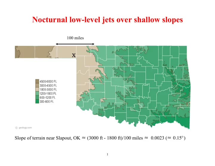
Nocturnal low-level jets over shallow slopes 100 miles x ¡ Slope of terrain near Slapout, OK ! (3000 ft - 1800 ft)/100 miles ! 0.0023 ( ! 0.15 ! ) 1

Blackadar (1957) inertial oscillation theory for LLJs Daytime Boundary layer characterized by dry-convective mixing. Get a 3-way balance between pressure gradient force (PGF), Coriolis force, and friction (turbulent stresses). Sunset Rapid stabilization of boundary layer. Dry-convective mixing ceases. Turbulent stresses shut down. Flow is now unbalanced: parcels accelerate (initially in direction opposite the daytime friction force). Nighttime Coriolis force deflects the unbalanced flow. Get an inertial oscillation (IO), an anticyclonically turning circular hodograph. 2

Schematic of an inertial oscillation (after Blackadar 1957) Curve OAB is daytime wind hodograph. Point B is the geostrophic wind at top of the boundary layer. The oscillation amplitude (radius R ) is equal to the initial (sunset) ageostrophic wind speed. 3

Maximum LLJ wind speed in the Blackadar scenario ! ! ! geos ageos wind = + wind wind At the ground (point O on Blackadar hodograph diagram) where the wind vector is 0 (no-slip), the ageostrophic wind is equal and opposite to the geostrophic wind (vector sum is 0). Thus, the largest possible value of the ageostrophic wind speed (and therefore largest possible R ) is the geostrophic wind speed. Thus, the largest LLJ wind speeds possible in the Blackadar scenario are twice the geostrophic wind speed. 4

Limitations of the Blackadar theory 1. The theory cannot explain how peak winds in some LLJs exceed geostrophic values by > 100% Wind speed vs height at Norman, OK from (a) 2331 UTC 6 July, (b) 0229 UTC 7 July, (c) 0535 UTC 7 July, (d) 0830 UTC 7 July, and (e) 1127 UTC 7 July (from Stensrud et al. 1990). 5

2. The theory cannot explain the geographical distribution of LLJs. LLJ frequency (from Bonner 1968) 6

LLJ frequency (from Walters et al. 2008) 7

3. Daytime winds vary with z less than in Blackadar schematic Peak ¡LLJ ¡ Daytime ¡ winds ¡in ¡ winds ¡in ¡ Blackadar ¡ Blackadar ¡ scenario: ¡ scenario: ¡ Peak ¡LLJ ¡ More ¡ winds ¡when ¡ realistic ¡ Blackadar-­‑like ¡ daytime ¡ theory ¡is ¡ winds: ¡ applied ¡to ¡ those ¡more ¡ realistic ¡ daytime ¡winds: Given realistic daytime wind profiles, a Blackadar-like theory would yield broad, weak and not-very-jet-like LLJs. 8

Holton (1967) sloping boundary layer theory for LLJs Viscous equations of motion and thermodynamic energy for a stably- stratified sloping boundary layer were solved analytically. Attention restricted to spatially and temporally constant southerly geostrophic wind, and an imposed periodic (monochromatic, T = 24 hr) volumetric radiative forcing. A diurnal wind oscillation was induced, but the results did not correctly reproduce the observed phase of the diurnal oscillations, and arguably the flow was not as jet-like as in observations. 9

Bonner and Paegle (1970) "sort-of" sloping boundary layer theory for LLJs Considered time-varying eddy viscosity and geostrophic wind. Periodicity of the geostrophic wind ascribed to diurnal temperature cycle over gently sloping terrain but analysis did not explicitly take terrain into account. Results were in reasonable agreement with observations, but amplitude of the oscillation was very sensitive to the magnitude of the geostrophic wind, choice of viscosity, and phase difference between the viscosity and the geostrophic wind. 10

Shapiro and Fedorovich (2009; SF09) Tilted Residual Layer theory of Great Plains LLJs Examined effects of terrain slope, thermal boundary layer structure, environmental stratification and synoptic-scale PGF on LLJ evolution. Considered a very simple framework: extended the inviscid, 1D Blackadar theory to include slope angle and a coupling between the equations of motion and thermodynamic energy. Treated LLJ as a response to the release of the frictional constraint near sunset, but considered the nature of the force(s) suddenly left unopposed to differ depending on a number of factors. Now let's examine this SF09 theory in detail. 11

Problem formulation Consider the development of a LLJ over a planar slope of infinite extent (no edges) having slope angle α . Work in slope-following Cartesian coordinates (as in our work with katabatic flow): v G ¡ ¡ y ¡ x ¡ α Restrict attention to (typical) case where synoptic-scale PGF points toward west, so geostrophic wind is southerly ( v G > 0), and treat f , v G , N as constant. Same restrictions considered by Holton (1967). 12

Governing equations du dt = ! b sin ! + f v ! f v G , (1) dv dt = ! fu , (2) db dt = u N 2 sin ! , (3) u , v are down- and cross-slope velocity components, respectively, b ! g ( " # " e )/ " r , where θ e is free-atmosphere potential temperature, N ! ( g / " r ) d " e / dz is Brunt-Väisälä frequency, v G is geostrophic wind, f is Coriolis parameter. Terms in blue not accounted for in original Blackadar theory. 13

Free-atmosphere N versus local stratification The N in (3) is environmental stratification. Local stratification will appear when we consider initial (sunset) conditions for parcel buoyancy. Free-atmosphere N appearance in (3) means downslope derivative of q within boundary layer is being set to downslope derivative of q at top of boundary layer, i.e., in free atmosphere. This scenario underpins many 1D slope flow models (Prandtl 1942, Gutman & Malbakhov 1964, Rao & Snodgrass 1981, McNider 1982, Sorbjan 1989, Grisogono & Oerlemans 2001, Shapiro & Fedorovich 2008). See also Fig. 12 of McNider and Pielke (1981). Free-atmosphere N term in (3) yields warming in presence of downslope flow, and cooling in presence of upslope flow. 14

Potential temperature over a heated slope (from numerical simulation of McNider and Pielke 1981) 15

Solution for the hodograph Use (2) to eliminate u in favor of v in (3), then integrate to get: v N 2 sin ! + b f = const . (4) Take u ! (1) + ( v – v G ,) ! (2) + b / N 2 ! (3), then integrate to get: ) 2 + b 2 u 2 + v ! v G N 2 = const . ( (5) Eliminating b between (4) and (5) yields u 2 + v 2 (1 + N 2 sin 2 ! / f 2 ) + mv = n , (6) where m and n are functions of the parameters (not shown). Equation (6) describes an ellipse with major axis along the u -axis and minor axis along the v -axis. The ratio of major to minor axes is 1 + N 2 sin 2 ! / f 2 . 16

2 1.5 1 V 0.5 0 -1 -0.5 0 0.5 1 U Hodographs of inertia-gravity oscillation over terrain at latitude 35 ° N with slope a = 0.2 ° for N =0 (dashed curve) and for N = 0.015s -1 (solid curve). Downslope ( U ) and cross-slope ( V ) wind components are normalized by geostrophic wind speed. Hodographs correspond to same initial conditions: B 0 = 0 , U 0 = 0 , and V 0 = 0.4 . 17

Predicted west/east elongation of LLJ hodographs is consistent with many observations of LLJs over the Great Plains. (from Zhong et al. 1996) 18

2 yr climatological hodograph from the Southern Great Plains Cloud and Radiation Testbed central facility in North-Central Oklahoma (from Whiteman et al. 1997) 19

6 yr climatological hodograph from Beaumont, KS (from Song et al. 2005) 20

Non-dimensionalization Define: Bu ! N 2 sin 2 " , the slope Burger number, f 2 ! " 1 + Bu . It is convenient to introduce the non-dimensional variables, B ! b sin " U ! u V ! v T ! ft , v G , v G , , f v G B 0 ! b 0 sin " U 0 ! u 0 V 0 ! v 0 . v G , v G , f v G 21

Analytical solution of (1)-(3) The solution for U , V , and B , expressed as deviations from their initial values is: ( + 1 U ( T ) ! U 0 = U 0 cos " T ! 1 " ! B 0 + V 0 ! 1 ( sin " T , (7) # & # & % % $ ' $ ' V ( T ) ! V 0 = ! U 0 " sin " T + 1 " 2 ! B 0 + V 0 ! 1 ( cos " T ! 1 ( , (8) # & # & % % $ ' $ ' B ( T ) ! B 0 = " 2 ! 1 U 0 sin " T ! " 2 ! 1 ! B 0 + V 0 ! 1 ( cos " T ! 1 ( . (9) # & # & " " 2 % % $ ' $ ' B 0 and V 0 on the right hand sides of the solutions (7)-(9) always appear in the combination ! B 0 + V 0 , so smaller initial southerly wind component (larger ageostrophic wind) is equivalent to larger positive initial buoyancy. 22

Reference values for slope angle α = 0 ° Flat terrain. Problem reduces to Blackadar scenario. α = 0.15 ° Characteristic slope of Texas/Oklahoma panhandles. Close to the 1/400 slope considered by Holton (1967). α = 0.5 ° Upper bound for the terrain slope of the far western Great Plains. α = 1 ° West of the Great Plains (i.e., in foothills somewhere) 23

Time series of U , V , B at latitude 35 ° N with N = 0.01s -1 with initial parcel buoyancy set to zero. Results shown for V 0 = 0.4 (solid lines) and V 0 = 0.8 (dashed lines). Initial values U 0 and B 0 were set to 0 . slope angle: 0 ° slope angle: 0.15 ° 2 0 2 0 B B 1.5 1.5 V -1 -1 V 1 1 U , V U , V B B 0.5 0.5 -2 -2 U 0 0 U -0.5 -0.5 -3 -3 0 1 2 3 4 5 6 0 1 2 3 4 5 6 T T 24

slope angle: 0.5 ° slope angle: 1.0 ° 2 0 2 0 B B 1.5 1.5 -1 -1 V 1 1 V U , V U , V B B 0.5 0.5 -2 -2 U 0 U 0 -0.5 -0.5 -3 -3 0 1 2 3 4 5 6 0 1 2 3 4 5 6 T T None of these results reveal a strong jet! Results indicate peak jet winds weaken with slope angle. 25