SLIDE 1 New Idea: NL-Means Filter (Buades 2005) New Idea: NL-Means Filter (Buades 2005)
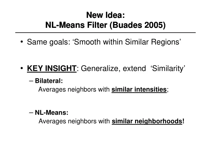
- Same goals: ‘Smooth within Similar Regions’
- KEY INSIGHT: Generalize, extend ‘Similarity’
– Bilateral:
Averages neighbors with similar intensities;
– NL-Means:
Averages neighbors with similar neighborhoods!
SLIDE 2 NL-Means Method: Buades (2005) NL-Means Method: Buades (2005)
every pixel p:
SLIDE 3 NL-Means Method: Buades (2005) NL-Means Method: Buades (2005)
every pixel p:
– Define a small, simple fixed size neighborhood;
SLIDE 4 NL-Means Method: Buades (2005) NL-Means Method: Buades (2005)
every pixel p:
– Define a small, simple fixed size neighborhood; – Define vector Vp: a list of neighboring pixel values.
Vp =
0.74 0.32 0.41 0.55 … … …
SLIDE 5
NL-Means Method: Buades (2005) NL-Means Method: Buades (2005)
‘Similar’ pixels p, q SMALL vector distance; || Vp – Vq ||2 p q
SLIDE 6
NL-Means Method: Buades (2005) NL-Means Method: Buades (2005)
‘Dissimilar’ pixels p, q LARGE vector distance; || Vp – Vq ||2 p q q
SLIDE 7
NL-Means Method: Buades (2005) NL-Means Method: Buades (2005)
‘Dissimilar’ pixels p, q LARGE vector distance; Filter with this! || Vp – Vq ||2 p q
SLIDE 8
NL-Means Method: Buades (2005) NL-Means Method: Buades (2005)
p, q neighbors define a vector distance; Filter with this:
No spatial term!
|| Vp – Vq ||2 p q
SLIDE 9
NL-Means Method: Buades (2005) NL-Means Method: Buades (2005)
pixels p, q neighbors Set a vector distance;
Vector Distance to p sets weight for each pixel q
|| Vp – Vq ||2 p q
SLIDE 10 NL-Means Method: Buades (2005) NL-Means Method: Buades (2005)
NL-Means maximizes the conditional probability
- f the central pixel given its neighborhood.
BF/WLS/RE assume the image is smooth. NL-Means assumes there are many repetitions in the image (i.e. the image is a fairly general stationary random process).
SLIDE 11 NL-Means Filter (Buades 2005) NL-Means Filter (Buades 2005)
source image:
SLIDE 12 NL-Means Filter (Buades 2005) NL-Means Filter (Buades 2005)
Filter Low noise, Low detail
SLIDE 13 NL-Means Filter (Buades 2005) NL-Means Filter (Buades 2005)
Diffusion (Note ‘stairsteps’: ~ piecewise constant)
SLIDE 14 NL-Means Filter (Buades 2005) NL-Means Filter (Buades 2005)
Filter (better, but similar ‘stairsteps’:
SLIDE 15 NL-Means Filter (Buades 2005) NL-Means Filter (Buades 2005)
Sharp, Low noise, Few artifacts.
SLIDE 16
NL-Means Filter (Buades 2005) NL-Means Filter (Buades 2005)
SLIDE 17
NL-Means Filter (Buades 2005) NL-Means Filter (Buades 2005)
SLIDE 18
NL-Means Filter (Buades 2005) NL-Means Filter (Buades 2005)
SLIDE 19 Isotropic Diffusion (Heat Equation)
The basic idea is simple: Embed the original image in a family of Derived images I(x,y,t) obtained by convolving the original image I_0(x,y) with a Gaussian kernel G(x,y;t) of variance t: I(x,t) = I_0(x,y)*G(x,y;t) This one parameter family of derived images may equivalently be viewed as the solution of the heat conduction, or diffusion, equation: With the initial condition I(x,y,0) = I_0(x,y), the original image.
SLIDE 20 Criteria for the Diffusion Equation
We would like diffusion to satisfy two criteria: 1) Causality: Any feature at a coarse level of resolution is required to possess a (not necessarily unique) “cause” at a finer level of resolution although the reverse need not be true. In other words, no spurious detail should be generated when the resolution is diminshed 2) Homogeneity and Isotropy: The blurring is required to be space invariant. The second criteria is not necessary, and as we shall see, using something else is a good idea!
SLIDE 21 Anisotropic Diffusion
divergence gradient Laplacian
This reduces to the isotropic heat diffusion equation if c(x,y,t)=const. Suppose we knew at time (scale) t, the location of region bounaries appropriate for that scale. We would want to encourage smoothing within a region in preference to smoothing across boundaries. This could be achieved by setting the conduction coefficient to be 1 in the interior of each region and 0 at the boundary. The problem: We don’t know the boundaries!
SLIDE 22 Criteria for the Anisotropic Diffusion Equation
We would like diffusion to satisfy three criteria: 1) Causality: Any feature at a coarse level of resolution is required to possess a (not necessarily unique) “cause” at a finer level of resolution although the reverse need not be true. In other words, no spurious detail should be generated when the resolution is diminshed 2) Immediate Localization. The boundaries should remain sharp and stable at all scales 3) Piecewise smooth: At all scales, intra-region smoothing should occur before inter-region smoothing. The second criteria is not necessary, and as we shall see, using something else is a good idea!
SLIDE 23 Solution: Guestimate!
Let E(x,y,t) be an estimate of edge locations. It should ideally have the following properties: 1)E(x,y,t) = 0 in the interior of each region 2)E(x,y,t) = Ke(x,y,t) at each edge point, where e is a unit vector normal to the edge at the point and K is the local contrast (difference in the image intensities on the left and right) of the edge If an estimate E(x,y,t) is available, then the conduction coefficient c(x,y,t) can be chosen to be a function c = g(||E||). According to the previous discussion, g(.) has to be nonnegative monotonically decreasing function with g(0)=1
SLIDE 24 Properties of AD
1) AD maintains the causality principle (proof omitted) 2) AD enhances edges Proof: w.l.o.g assume the edge is aligned with y axis: And we choose c to be a function of the gradient of I: c(x,y,t) = g(I_x(x,y,t)). Let (I_x) = g(I_x) I_x denote c I_x (known as flux) Then, the 1D version of equation (3) becomes: We are interested in the variation in time of the slope of the edge: We want it to increase for strong (real) edge and decrease for weak (probably noise) edges.
SLIDE 25 Edge Enhancement
Given that I is smooth, we can invert the order of differentiation
Suppose the edge is oriented in such a way that I_x>0. At the point of inflection I_xx=0, and I_xxx<<0 since the point of inflection corresponds to the point with maximum slope. Then in a neighborhood of the point of inflection has sign opposite to ’(I_x) That’s because ’’(I_x)=0 at the point of inflection. So, if ’(I_x)>0 the slope of the edge will decrease in time; if ’(I_x)<0 the slope will increase with time
SLIDE 26
The choice of function () that leads to edge enhancement When increases, its derivative is greater than zero and the edge will get blurred. At some point, decreases and the edge will be enhanced. The g functions used in the paper are:
SLIDE 27 Implementation
Discretizing equation: Leads to (a discrete Laplacian equation): And the conduction coefficients are:
SLIDE 28
Results
SLIDE 29
Results
SLIDE 30
Results
SLIDE 31 Robust statistics is about dealing with outliers Within the context of image denoising, edges are
- utliers, because if we had no edges then a simple
Gaussian blur would do the job. Formally, we want to minimize: That is, every pixel s should be close to its neighbors p This objective function can be solved with the following gradient descent scheme: where Anisotropic Diffusion, Robust Statistics and Line Process
SLIDE 32
The Quadratic Error Norm
SLIDE 33
The Lorenzian Error Norm
SLIDE 34 The connection between AD and RS
Anisotropic Diffusion: By defining: we get equivalence between the two approaches. In the discrete case we have: Robust Statistics Objective Function Gradient Descent with
SLIDE 35 Example
Perona-Malik suggest: For a positive constant K. We want to find a \rho() function such that the iterative solution of the diffusion equation and the robust statistics equation are equivalent. Letting we have:
SLIDE 36
PM and the Lorenzian
SLIDE 37 Tukey’s biweight
Why settle for the Lorenzian? Maybe we can choose a more robust error measure?
SLIDE 38 Or Huber’s minimax norm?
Huber’s minimax norm is equivalent to the L_1 norm for large values. But, for normally distributed data, the L_1 norm produces estimates with higher variance than the optimal L_2 (quadratic) norm, so Huber’s minmax norm is designed to be quadratic for small values
SLIDE 39 Comparing all three functions
Now we can compare the three error norms directly. The modified L_1 norm gives all outliers a constant weight of one while the Tukey norm gives zero weight to outliers whose magnitude is above a certain value. The Lorentzian (or Perona-Malik) norm is in between the other two. Based
- n the shape of the influence function \psi() we would correctly predict that diffusing with the
Tukey normproduces sharper boundaries than diffusing with the Lorentzian (standard Perona-Malik) norm, and that both produce sharper boundaries than the modified L1 norm
SLIDE 40
Results
SLIDE 41
Results
SLIDE 42
Results
SLIDE 43 Robust Statistics Line Processes
Robust estimation minimizes: Where Equivalently, we can formulate the following line process minimization problem:
where
One benefit of the line-process approach is that the “outliers” are made explicit and therefore can be manipulated. As we will see shortly
SLIDE 44 Line Process of Lorenzian (Perona-Malik)
Our goal is to take a function (x) and construct a new function, E(x;l)=(x^2l+P(l)), such that the solution at the minimum is unchanged In the case of the Lorentzian norm, it can be shown that P(l) = l-1-log(l) And the line equation becomes: Differentiating with respect to I_s and l gives the following iterative equations for minimizing:
SLIDE 45 Adding spatial priors
We consider two kinds of interaction terms, hysteresis and non-maximum suppression. Other common types of interactions (for example corners) can be modeled in a similar way. The hysteresis term assists in the formation of unbroken contours while the non-maximum suppression term inhibits multiple responses to a single edge present in the data. Hysteresis lowers the penalty for creating extended edges and non-maximum suppression increases the penalty for creating edges that are more that one pixel wide.
We define a new term that penalizes the configurations on the right of the figure and rewards those on the left. This term, E_I, encodes our prior assumptions about the organization of spatial discontinuities where the parameters \epsilon_1 and \epsilon_2 assume values in the interval [0;1] and \alpha controls the importance of the spatial interaction term.
SLIDE 46 Putting it all together
Starting with the Lorentzian norm, the new error term with constraints on the line processes becomes Where Differentiating this equation with respect to I and l gives the following update equations: The value of the line process at each point is taken to be the product, l_{s,h}*l_{s,v} of the horizontal and vertical line processes.
SLIDE 47 Effect of Line process priors
SLIDE 48 Example on real image