NIRT: Coherence and Correlation in Electronic Nanostructures (Duke - - PDF document

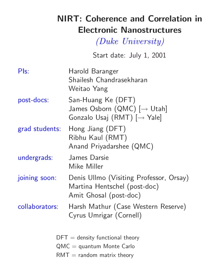
NIRT: Coherence and Correlation in Electronic Nanostructures (Duke University)

Start date: July 1, 2001 PIs: Harold Baranger Shailesh Chandrasekharan Weitao Yang post-docs: San-Huang Ke (DFT) James Osborn (QMC) [→ Utah] Gonzalo Usaj (RMT) [→ Yale] grad students: Hong Jiang (DFT) Ribhu Kaul (RMT) Anand Priyadarshee (QMC) undergrads: James Darsie Mike Miller joining soon: Denis Ullmo (Visiting Professor, Orsay) Martina Hentschel (post-doc) Amit Ghosal (post-doc) collaborators: Harsh Mathur (Case Western Reserve) Cyrus Umrigar (Cornell)

DFT = density functional theory QMC = quantum Monte Carlo RMT = random matrix theory

1

Motivation

• I. Quantum Dots

confinement ⇒ interference confinement ⇒ interactions ( charging + residual) ⇒ interplay between interactions and interference spin of dot?? − → spintronics ... quantum computing ...

100 − 1000 electrons [Marcus group]

• II. Molecular Electronics

single molecule attached to leads

• I-V curve?
• non-equilibrium effects?
• Kondo effect recently observed!

Vg V

[Ralph and McEuen groups]

• III. Nano– Magnetism, Superconductivity, ...

strong e-e interactions + confinement/disorder

• fluctuation of anisotropy energy in magnetic nanoparticles
• superconductor-insulator transition disordered metal films
• metal-insulator transition in disordered 2DEG

Outline

• I. Random Matrix Theory Description of Quantum Dots
• Coulomb blockade (CB) conductance peaks

− → fluctuation of ground state energy and spin

• the “universal Hamiltonian”
• CB peak spacing distribution agrees with experiment
• II. Density Functional Theory of Quantum Dots
• 2D LSDA calculation for isolated quantum dots

3D calculation with real gate configuration coming soon...

• Addition energy for up to 200 electrons – large N matters!
• Interaction effects much stronger than expected
• III. Quantum Monte Carlo Study of Disorder in Superconductivity
• modified Hubbard model: localization ⇐

⇒ strong e-e interactions

• Kosterlitz-Thouless in clean; Superconductor-Insulator in dirty
• exponential decay of pair correlations for arbitrarily small disorder!

Spacing of Coulomb Blockade Conductance Peaks

Gonzalo Usaj, Denis Ullmo, and H.B.

• weakly coupled dot

⇒ N is well defined

• N →N +1 costs energy

∼e2/C ⇒ blockade.

• EN(V ∗

g )=EN+1(V ∗ g )

⇒ G peaks.

[Patel et al.]

EN

GS − eN Cg

C V ∗

g =EN+1 GS

− e(N + 1)Cg C V ∗

g

• peak position V ∗

g ∝ EN+1 GS −EN GS

= ⇒ spacing ∝ (EN+1

GS

−EN

GS) − (EN GS−EN−1 GS

)

• Fluctuation of spacing ⇔ Fluctuation of GS energy of the dot.

An effective Hamiltonian

• only energy levels around the Fermi energy are relevant
• chaotic dynamics → RMT for single-particle properties (energy window up to Eth ∼ ¯

h/tflight)

• Screening is important ⇒ weak interaction

Vsc(r1, r2)= e2 C +VTF(r1, r2)+V (r1)∆+V (r2)∆ ⇓ ˆ Hint=EC ˆ n2+ˆ n

• α,β,σ

c†

α,σcβ,σ Xα,β + 1

2

• α,β,γ,δ

Hα,β,γ,δ c†

δ,σc† γ,σ′cβ,σ′cα,σ

Hα,β,γ,δ =

• dr1dr2Ψ∗

δ(r1)Ψ∗ γ(r2)VTF(r1−r2)Ψβ(r2)Ψα(r1)

Xα,β =∆

• drV (r)Ψ∗

α(r)Ψβ(r)

• Fluctuations Ψα(r) ⇒ fluctuations Hα,β,γ,δ and Xα,β
• Fluctuations are small ⇒ controlled by 1/kF

√ A (or 1/g, g = Eth/∆) .

⇒ expand ˆ Hint in powers of 1/g

[Blanter, Mirlin, Muzykanskii; Aleiner, Brouwer, Glazman; Altshuler]

CEI model (g → ∞)

Large N limit ⇒ Hα,β,γ,δ = J′ δα,δδβ,γ + JS δα,γδβ,δ dominates ⇒ HCEI =

• α,σ

ǫα ˆ nα,σ + EC(ˆ n − N)2−JS S2

[Kurland, Aleiner,Altshuler]

• JS <

∼ ∆/2 ⇒ main reason CI model is wrong

• Interplay of JS and {ǫα} ⇒ S = 1 if ∆1 − 2JS < 0

∆1

• 0.5

0.5 1 1.5

spacing [∆]

0.5 1 1.5 2

Probability Density

• 0.5

0.5 1 1.5

even

• dd

0.5 1 1.5 S 0.5 1 P(S) 0.5 1 1.5 0.5 1 0.79 0.99 0.21 0.01

rs ∼ 1 ⇒ Js ≈ 0.3∆

[Ullmo, Baranger]

5

Experiment Theory

• 1.0
• 0.5

0.0 0.5 1.0 Spacing (∆) 0.0 0.5 1.0 1.5 2.0 Probability Distribution P(s)

"Odd" "Even"

• 0.5

0.5 1

spacing [∆]

1 2 3 4

Probability density

• 0.5

0.5 1

kBT = 0.3∆ r.m.s. = 0.235∆

even

• dd

[Patel et al.; Ong et al.]

Theory includes leading corrections to CEI model + temperature

• “scrambling”: added electron changes mean-£eld potential and so {ǫi}
• “gate effect”: gate voltage which increases N also changes interference
• residual interactions: fluctuations of diagonal terms in Hα,β,γ,δ
• kBT: compare to ∆ − 2Js −

→ important! Note: even/odd effect, no δ-function, large spacing tail in even

T = 0 PSD: including corrections

• 0.5

0.5 1 1.5

spacing [∆]

0.5 1 1.5 2

Probability density

• 0.5

0.5 1 1.5 0.5 1 1.5 2

kBT = 0.1∆ r.m.s. = 0.286∆

• 0.5

0.5 1 1.5

spacing [∆]

0.5 1 1.5 2

Probability density

• 0.5

0.5 1 1.5 0.5 1 1.5 2

kBT = 0.3∆ r.m.s. = 0.235∆

even

• dd
• Notice double peak structure at low T
• At kBT ∼ 0.3∆, temperature effect dominates

⇒lower T experiments are needed!

Density Functional Study of CB in Quantum Dots

Hong Jiang, Weitao Yang, and H.B. 2D Model System: V (x, y) = a x4 b + by4 + 2λx2y2 + γ(x2y − xy2)

• 20
• 10

10 20

• 20
• 10

10 20

1 2 3 4

Spacing

0.2 0.4 0.6 0.8

Distribution

Calculated NNS distribution Wigner GOE distribution

a = 1.0 × 10−4, b = π

4

λ = −0.6, γ = 0.0 Nearest neighbouring spacing distribution for single-particle spectrum in 1 symmetry class.

Computational Techniques

DFT-Kohn-Sham Method for e-e interaction

• − ¯

h2 2m∗ ∇2 + e2 κ

• ρ(r′)

|r−r′|dr′ + δExc[ρ,ζ] δρσ(r)

+ Vext(r)

• ψσ

i (r) = ǫσ i ψσ i (r)

• 2D Local-spin density approximation (LSDA) and

Tanatar-Ceperley parameterized form for exchange-correlation functional;

• Fast-sine transform for kinetic energy operator, and real space

representation of wave functions;

• Preconditioned conjugate-gradient method for Kohn-Sham

equations.

• Fast-Fourier transform method for Hartree potential

3

Data Analysis: Fitting

50 100 150 200

Electron Number

0.05 0.07 0.09 0.11 0.13 0.15 0.17 0.19

Addition Energy

Raw data and fitting

Polynomial Fitting Raw Data 50 100 150 200

Electron Number

−0.02 −0.01 0.01 0.02

Addition Energy

Smooth part removed.

6

0.5 1 1.5

1 2 0.5 1 2 0.5 1 2 0.5

• 1

1 2 0.5 1 1.5

1 2 0.5

• 1

1 2

1 2 0.5

• 1

1 2

1 2 0.5

(a) (b) (c) (d) (e) (f)

Probability Density

Asymmetric N=20-80 N=80-140 N=140-200

Spacing

P(S) P(S) P(S) P(S) P(S) P(S) Symmetric

• 2D LSDA model of isolated quantum dot with chaotic external potential
• Statistical properties of addition energy for up to 200 electrons
• Electron number matters!
• Symmetry matters!

Why are interactions so strong??

Disorder Induced Superconductor-Insulator Transition

James Osborn, Shailesh Chandrasekharan, and H.B. A Modified Hubbard Model: H =

• <i,j>
• σ (c†

i,σcj,σ + c† j,σci,σ) (ni + nj − 1)(ni + nj − 3) + 2

Si · Sj + 2 Ji · Jj − 4

• ni,↑ − 1

2 ni,↓ − 1 2 nj,↑ − 1 2 nj,↓ − 1 2

• +
• i
• U
• ni,↑ − 1

2 ni,↓ − 1 2

• − µi ni
• with

ni = ni,↑ + ni,↓ and J+

i = (−1)i c† i,↑ c† i,↓ ,

J−

i = (−1)i ci,↓ ci,↑ ,

J3

i = 1

2 (ni,↑ + ni,↓ − 1) Disorder: µi = µ + Wri with −1 < ri < 1.

• Same symmetries as standard Hubbard model:

SU(2) spin; SU(2) charge broken by µ to U(1) number

• Shows s-wave superconductivity for U ≤ 0

(except at half-filling where antiferromagnetism is stable)

• Not free for U = 0.

= ⇒ Localization ← → Strong e-e Interactions

Superfluid Density vs. Disorder β = 5

1 2 3 4 disorder (W) 1 2 3 4 5 6 7 8 2 π ρs / T L = 8 L = 16 L = 24 L = 32

ρs ≡ T 4

• (Wx/2)2 + (Wy/2)2

where Wx is the total number of particles winding around the boundary in the x direction In the clean case, 2π T ρs = 2 + √ A coth( √ A log(L/L0)) for T < Tc with A = 0 at T = Tc.

Pair Susceptibility vs. Length β = 5

8 16 32 64 128 L 100 1000 10000 pair susceptibility W = 0 W = 0.05 W = 0.1

χL = 1 ZV

β 0 dt Tr

• e−(β−t)H (∆† + ∆) e−tH (∆† + ∆)
• with ∆ ≡
• x cx,↓ cx,↑

In the clean case for T < Tc, χL ∝ L2−η(T) with η(Tc) = 1/4 and η(0) = 0

Pair Susceptibility vs. Disorder β = 5

1 2 3 4 disorder 10 100 1000 10000 pair susceptibility 1 2 3 4 10 100 1000 10000 L = 128 L = 96 L = 64 L = 32 L = 16 L = 8 0.1 0.2 0.3 0.4 0.5 5000 10000 15000 5000 10000 15000