ni Txizx ] " Independence, Continued Example: Max of Two - - PowerPoint PPT Presentation

ni
SMART_READER_LITE
LIVE PREVIEW

ni Txizx ] " Independence, Continued Example: Max of Two - - PowerPoint PPT Presentation

Not Too Different From Discrete... A Note on Independence For continuous RVs, what is weird about the Continuous RVs Continued: Discrete RV: following? X and Y are independent iff for all a , b : Independence, Conditioning, P [ X = a , Y = b ]


slide-1
SLIDE 1

Continuous RVs Continued: Independence, Conditioning, Gaussians, CLT

CS 70, Summer 2019 Lecture 25, 8/6/19

1 / 26

Not Too Different From Discrete...

Discrete RV: X and Y are independent iff for all a, b: P[X = a, Y = b] = P[X = a] · P[Y = b] Continuous RV: X and Y are independent iff for all a ≤ b, c ≤ d: P[a ≤ X ≤ b, c ≤ Y ≤ d] =

2 / 26

Plas

X Eb ]

x IPCC EYE

d ]

A Note on Independence

For continuous RVs, what is weird about the following? P[X = a, Y = b] = P[X = a] · P[Y = b] What we can do: consider a interval of length dx around a and b!

3 / 26

  • To

To

=

O

IPCX

  • a , Y
  • b)

=p f X Efa ,

atdx

)

, YE [ b.

btdy ))

=

PEX E Ca ,

at DX) ) REY E [ b

, btdy

=

ffx(a) dxlffyl

b) dy)

Independence, Continued

If X, Y are independent, their joint density is the product of their individual densities: fX,Y (x, y) = Example: If X, Y are independent exponential RVs with parameter λ:

4 / 26

fxlx )

. fy

C y )

f × , y ( X

, y ) =

f x ( x )

  • f

y ( y )

=

(

xe

  • xxxx

e

  • M )
=

He

  • XCX ty )

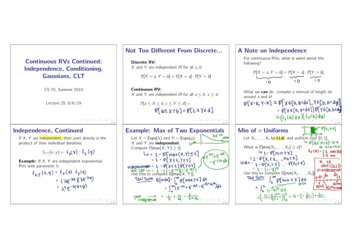
Example: Max of Two Exponentials

Let X ∼ Expo(λ) and Y ∼ Expo(µ). X and Y are independent. Compute P[max(X, Y ) ≥ t]. Use this to compute E[max(X, Y )].

5 / 26

'

is

:

=

I

  • lpfmaxcx
, Y)

Et ]

  • ut
=

I

  • IP [ X

Et

, YET ]

indecencies

:

:

¥¥E¥¥

,

Tails

:

Efmaxt

  • fo
  • p[

maxzt

]

dt

= So
  • ( e
  • atte
  • Ut
  • e-

HUH )dt

poftiegra.TN

=

at

  • 1 tu
  • life

Min of n Uniforms

Let X1, . . . , Xn be i.i.d. and uniform over [0, 1]. What is P[min(X1, . . . , Xn) ≤ x]? Use this to compute E[min(X1, . . . , Xn)].

6 / 26

!

"

Txizx ]

↳ IPCAEXEBT

  • b
  • a

for

OEAEBEI ↳

1-

IPC

minzx

]

fxtx

)

  • {

I

  • verlay

=L

  • IPCX ,

2X

, . . . ,

Xnzx

]

° aw

.

in

.

ni

" "

"

" ' '

÷÷÷iL¥÷

Tailsvm

:

So

  • lpcmin

ZXIDX

iefmax

= got

y

prer

.

( I

  • X

)ndx

'

ECmin%ECzndsmanesty-f.a-xn.IT#I--o-tnttiI--nt

slide-2
SLIDE 2

Min of n Uniforms

What is the CDF of min(X1, . . . , Xn)? What is the PDF of min(X1, . . . , Xn)?

7 / 26

from prev

Fmln l X )

= BE

mine

× ]

=

z

. , , .

xfgn slide

d

Tx

C I

  • CI
  • Xin )

O

  • n ( I
  • X )

n

  • tf

1)

f-min

#

Nfl

  • x )

n

  • I

Memorylessness of Exponential

We can’t talk about independence without talking about conditional probability! Let X ∼ Expo(λ). X is memoryless, i.e. P[X ≥ s + t|X > t] = P[X ≥ s]

8 / 26

LHS

:

p

zsttfnfxstpredundant-pxteventj-f.ie

=

lpfxzstt ]

Pasty

=

e- Htt )

T

etat

=

e-

7S=p[

XZS ]

Conditional Density

What happens if we condition on events like X = a? These have 0 probability! The same story as discrete, except we now need to define a conditional density: fY |X(y|x) = fX,Y (x, y) fX(x) Think of f (y|x) as P [Y 2 [y, y + dy]|X 2 [x, x + dx]]

9 / 26

convention

:

set this too when f

× ( X )

'
  • O
.

YIX

Conditional Density, Continued

Given a conditional density fY |X, compute P[Y ≤ y|X = x] = If we know P[Y ≤ y|X = x], compute P[Y ≤ y] = Go with your gut! What worked for discrete also works for continuous.

10 / 26

Cy , ytdy ]

a

  • pCY=yTx=

;D

Iffy.KZ/X)dz

Cxxtdx

1%1 ysylx

  • XTfxtxdxotpafb.ru
.

I

If discrete

:

case

  • n

x !

§

PETEY IX

  • X ]
. PEX
  • I

Example: Sum of Two Exponentials

Let X1, X2 be i.i.d Expo(λ) RVs. Let Y = X1 + X2. What is P[Y < y|X1 = x]? What is P[Y < y]?

11 / 26

↳ ±¥i¥¥¥7EE¥ case

  • n

values for

Xi !

jipfyeylx

,

x )

. IPCX ,
  • X ]

1%1

  • e-

" Y

  • X ')f×¥dx

I

Soya

  • e
  • Hy
  • x ) )

a e

  • xxdx
.

Exercise

.

Example: Total Probability Rule

What is the CDF of Y ? What is the PDF of Y ?

12 / 26

Exercise

I I
slide-3
SLIDE 3

Break

If you could immediately gain one new skill, what would it be?

13 / 26

The Normal (Gaussian) Distribution

X is a normal or Gaussian RV if: fX(x) = 1 p 2πσ2 · e(x−µ)2/2σ2 Parameters: Notation: X ∼ E[X] = Var(X) = Standard Normal:

14 / 26

* SY

mm

.

About

#

its

mean

if

,

O

Ncel

,

02 ) 02

U

µ=o

,

02=1

¥17

Gaussian Tail Bound

Let X ∼ N(0, 1). Easy upper bound on P[|X| ≥ α], for α ≥ 1? (Something we’ve seen before...)

15 / 26

Chebyshev

:

FPC Ix

  • of

za ]

s VarC

±

I

42

Gaussian Tail Bound, Continued

Turns out we can do better than Chebyshev. Idea: Use R 1

α 1 p 2πe−x2/2dx ≤

16 / 26

SETTEE

  • Mdx

N

pflXH2]=2lP[XZx ]

¥19

=2SIfae-×%dx

shaded

:

Hkd

⇐ 210¥

,e-X%dX

2k¥ .lk#X-iDl :

I

Shifting and Scaling Gaussians

Let X ∼ N(µ, σ) and Y = X−µ

σ . Then:

Y ∼ Proof: Compute P[a ≤ Y ≤ b]. Change of variables: x = σy + µ.

17 / 26

2

NCO

,

I)

Notes

:
  • ut
  • f

scope

.

Shifting and Scaling Gaussians

Can also go the other direction: If X ∼ N(0, 1), and Y = µ + σX: Y is still Gaussian! E[Y ] = Var(Y ) =

18 / 26

ECU

to

XI

=

if

to EAT

° =

if

Var ( y

to X )

=

Var fo X )

=
  • 2

Var ( X)

=

f

2

slide-4
SLIDE 4

Sum of Independent Gaussians

Let X, Y be independent standard Gaussians. Let Z = [aX + c] + [bY + d]. Then, Z is also Gaussian! (Proof optional.) E[Z] = Var(Z) =

19 / 26

ECaxtctbytdf.at#yIIoaECY7/--ctdVar(aXtbYtCtd)--Var(aXtbY

)

I shift

=

Varcax ) tvarcby

)

=

azvarcx )

tbzvarcy

)

=

a2tb2

Example: Height

Consider a family of a two parents and twins with the same height. The parents’ heights are independently drawn from a N(65, 5) distribution. The twins’ height are independent of the parents’, and from a N(40, 10) distribution. Let H be the sum of the heights in the family. Define relevant RVs:

20 / 26

Exercise

Example: Height

E[H] = Var[H] =

21 / 26

Sample Mean

We sample a RV X independently n times. X has mean µ, variance σ2. Denote the sample mean by An = X1+X2+...+Xn

n

E[X] = Var(X) =

22 / 26

An

Eftncxit

. .

.tl/nD=tn(ECX.It:.tEEXnD--tnfnu)--UAnVarftnCXit...tXnD--

ntzfyarCXD.it

. . .

tvarcxn )]

=

'#fAo4=

In

The Central Limit Theorem (CLT)

Let X1, X2, . . . , Xn be i.i.d. RVs with mean µ, variance σ2. (Assume mean, variance, are finite.) Sample mean, as before: An = X1+X2+...+Xn

n

Recall: E[An] = Var(An) = Normalize the sample mean: A0

n =

Then, as n ! 1, P[A0

n] !

23 / 26

it

%

An

  • µ

f

Standdeairadtion

normalized

  • sammpleean
.

Ern 3

An

'

as n

→ A

=

follows

A

easier

WAY

:

Ncaa )

dist

.

Example: Chebyshev vs. CLT

Let X1, X2, . . . be i.i.d RVs with E[Xi] = 1 and Var(Xi) = 1

  • 2. Let An = X1+X2+...+Xn

n

. E[An] = Var(An) = Normalize to get A0

n:

24 / 26

1 02

a-

=If

ECA'n7=EfAn]=

Ende

:

Var

( A

'

n )

=

Var (

An

  • 1

this !

C- expectation

  • f

single

sample

.

variance

  • f

a

single

sample

  • An
  • IE CAN]
  • tartan
slide-5
SLIDE 5

Example: Chebyshev vs. CLT

Upper bound P[A0

n ≥ 2] for any n.

(We don’t know if A0

n is non-neg or symmetric.)

If we take n ! 1, upper bound on P[A0

n ≥ 2]?

25 / 26

Plan

'

22 ] E

1pct An

'
  • of

22 ]

s

variant

T

22

ECA n' I

s tf

Gaussian

tail

him

PEA 'm

22 ]

E

const

X

e

  • 2%
=

const

't #

I ②

68

  • 95-99.7

approaches

195%

Nco

. 1)

dist

. ±¥9%¥Eao£

"

" "

Summary

I Independence and conditioning also generalize from the discrete RV case. I The Gaussian is a very important continuous

  • RV. It has several nice properties, including

the fact that adding independent Gaussians gets you another Gaussian I The CLT tells us that if we take a sample average of a RV, the distribution of this average will approach a standard normal.

26 / 26