Neural-Symbolic Integration Strategies Neural-Symbolic Integration - - PowerPoint PPT Presentation

Neural-Symbolic Integration Strategies

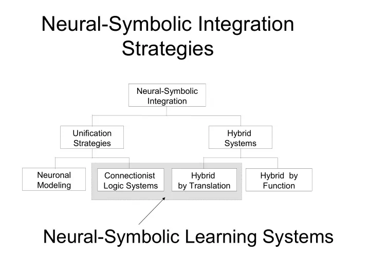
Neuronal Modeling Connectionist Logic Systems Hybrid by Translation Hybrid by Function Hybrid Systems Unification Strategies Neural-Symbolic Integration

Neural-Symbolic Learning Systems

CILP: Connectionist Inductive Logic Programming System

Objective: To benefit from the integration of

Artificial Neural Networks and Symbolic Rules.

C ← F, ~G; F ← A ← B,C,~D; A ← E,F; B ←

Exploiting Background Knowledge Explanation Capability Efficient Learning Massively Parallel Computation

CILP structure

• 1. Adding Background Knowledge (BK)
• 2. Computing BK in Parallel
• 3. Adding Training with Examples
• 4. Extracting Knowledge
• 5. Closing the Cycle

Symbolic Knowledge Symbolic Knowledge Neural Network Examples

Learning Connectionist System

Inference Machine

Explanation

1 3 2 4 5

Theory Refinement Contents

 Inserting Background Knowledge  Performing Inductive Learning with

Examples

 Adding Classical Negation  Adding Metalevel Priorities  Experimental Results

Inserting Background Knowledge

A B

θ A θ B

W W W

θ 1 N 1 θ 2 N2 θ 3 N 3

B F E D C W W W

• W

W

Int er pr etatio ns

Example: P = { A ← B,C,~D; A ← E,F; B ← }

General clause: A0 ← A1…Am, ~Am+1 … ~ An

Theorem: For each general logic program P, there

exists a feedforward neural network N with exactly one hidden layer and semi-linear neurons such that N computes TP.

Corollary (analogous to [Holldobler and Kalinke

94]): Let P be an acceptable general program. There exists a recurrent neural network Nr with semi-linear neurons such that, starting from an arbitrary initial input, Nr converges to the unique stable model of P.

Inserting Background Knowledge

Wr = 1 A B

• (1+A min )W/2

W W W W W N1 N3 N2 (1+A min )W (1+A min )W/2 W W W

• W

T F E D C B Interpretations 1

Example: P = { A ← B,C,~D; A ← E,F; B ← }. Recurrently connected, N converges to stable state: {A = false, B = true, C = false, D = false, E = false, F = false}

Computing with Background Knowledge

• 1

1 Amin Amax

CILP translation algorithm

W > 2 (ln(1+Amin) – ln(1-Amin)) / (max(k,m).(Amin-1)+Amin+1)

Produces neural network N given logic program P N can be trained with backpropagation subsequently Given P with clauses of the form: A if L1, ..., Lk Let p be the number of positive literals in L1, ..., Lk Let m be the number of clauses in P with A in the head Amin denotes the minimum activation for a neuron to be true Amax denotes the maximum activation for a neuron to be false

Θh = (1+Amin).(k-1).W/2 (threshold of hidden neuron) ΘA = (1+Amin).(1-m).W/2 (threshold of output neuron) Amin > max(k,m)-1 / max(k,m)+1 Amax = -Amin (for simplicity)

• Neural Networks may be trained with examples to

approximate the operator TP associated with a Logic Program P.

• A differentiable activation function, e.g. the bipolar

semi-linear function h(x) = (2 / (1 + e-x)) - 1, allows efficient learning with Backpropagation.

Performing Inductive Learning with Background Knowledge

Performing Inductive Learning with Background Knowledge

 We add extra input, output and hidden

neurons, depending on the application

 We fully-connect the network  We use Backpropagation

Adding classical negation

General Program: Cross ← ~ Train School bus crosses rail line in the absence

• f proof of approaching

train Extended Program: Cross ← ¬ Train School bus crosses rail line if there is proof of no approaching train

Extended clause: L0 ← L1…Lm, ~Lm+1 … ~ Ln

The Extended CILP System

B

¬ C

B

¬ C

D A

¬ E

N1 N3 N2 W W W

• W
• W

W W W

r1: A ← B, ¬C; r2: ¬C ← B, ~ ¬E; r3: B ← ~D

Adding Classical Negation

Theorem: For each extended logic program

P, there exists a feedforward neural network N with exactly one hidden layer and semi-linear neurons such that N computes TP.

Corollary: Let P be a consistent acceptable

extended program. There exists a recurrent neural network Nr with semi- linear neurons such that, starting from an arbitrary initial input, Nr converges to the unique answer set of P.

Example: P = { B ← ~ C; A ← B, ~ ¬ D; ¬ B ← A }. Recurrently connected, N converges to stable state: {A = true, B = true, ¬ B = true, C = false, ¬ D = false}

Computing with Classical Negation

N1 W

• W

W

• W

W W W N2 A B ¬B C B ¬D A N3

Adding Metalevel Priorities

r1 > r2 = “ x is preferred over ¬x ”, i.e. when r1 fires it should block the output of r2

a x r2 r1 b c d e ¬x

• nW

W

Learning Metalevel Priorities

r1 r2 r3 guilty ¬ guilty fingertips alibi super-grass

P = { r1: guilty ← fingertips, r2: ¬guilty ← alibi, r3: guilty ← supergrass }

Training examples include: [(-1, 1, *), (-1, 1)] [( 1, *, *), ( 1, -1)] where * means “don’t care”

r1 > r2 > r3

Learning Metalevel Priorities

r1 r2 r3 guilty ¬ guilty fingertips alibi super-grass

Wguilty, r1 = 3.97, Wguilty, r2 = – 1.93, W¬guilty, r1 = – 1.93 Wguilty, r3 = 1.94, W¬guilty, r2 = 1.94 W¬guilty, r3 = 0.00

θguilty = – 1.93, θ¬guilty = 1.93 r1 > r2 > r3 ?

Setting Linearly Ordered Theories

Wguilty,r3 = W Wguilty,r2 = – W + δ Wguilty,r1 = Wguilty,r3 – Wguilty,r2 + δ = 2W If W = 2, δ = 0.01: W guilty,r3 = 2 W guilty,r2 = – 1.99 W guilty,r1 = 4

• 3 < θguilty < 1
• 1 < θ¬guilty < 3

r1 r2 r3 guilty ¬ guilty fingertips alibi super-grass

r1 > r2 > r3

Partially Ordered Theories

r2 > r1 r3 > r1 r4 > r1

Each of r2 , r3 and r4 should block the conclusion of r1

r1 r2 r3 r4

X ¬X

Problematic Case

layEggs(platypus) monotreme(platypus) hasFur(platypus) hasBill(platypus) r1: mammal(x) ← monotreme(x) r2: mammal(x) ← hasFur(x) r3: ¬ mammal(x) ← layEggs(x) r4: ¬ mammal(x) ← hasBill(x)

r1 > r3 r2 > r4

Cannot have r1 > r3, r2 > r4 without also having r1 > r4 and r2 > r3

CILP Experimental Results

 Test Set Performance (how well it

generalises)

 Test Set Performance over small/increasing

training sets (how important BK is)

 Training Set Performance (how fast it trains)

CILP Experimental Results

• Promoter Recognition:

♦ A short DNA sequence that preceeds the beginning of

genes.

Background Knowledge

Promoter ← Contact, Conformation Contact ← Minus10, Minus35 Minus 10

← @ -14 ‘tataat’

Minus 10

← @ -13 ‘ta’, @ -10 ‘a’, @ -8 ‘t’

Minus 10

← @ -13 ‘tataat’

Minus 10

← @ -12 ‘ta’, @ -7 ‘t’

Minus 35

← @ -37 ‘cttgac’

Minus 35

← @ -36 ‘ttgac’

Minus 35

← @ -36 ‘ttgaca’

Minus 35

← @ -36 ‘ttg’, @ -32 ‘ca’

Conformation

← @ -45 ‘aa’, @ -41 ‘a’

Conformation ← @ -45 ‘a’, @ -41 ‘a’, @ -28 ‘tt’, @ -23 ‘t’, @ -21 ‘aa’, @ -17 ‘t’, @ -15 ‘t’, @ -4 ‘t’ Conformation ← @ -49 ‘a’, @ -44 ‘t’, @ -27 ‘t’, @ -22 ‘a’, @ -18 ‘t’, @ -16 ‘tg’, @ -1 ‘a’ Conformation ← @ -47 ‘caa’, @-43 ‘tt’, @-40 ‘ac’, @-22 ‘g’, @-18 ‘t’, @-16 ‘c’, @-8 ‘gcgcc’, @-2 ‘cc’

An Example Bioinformatics Rule

a

Minus5 . . . @-1 @5 @1

a g t c a g t c a g t c

Minus5 ← @-1'gc', @5't'

Promoter Recognition

53 examples of promoters 53 examples of non

• promoters

Initial Topology of the Network

Minus35 Minus10 Conform. Contact Promoter

• 50 DNA

+7 Minus35 Minus10 Conform. Contact

Test Set Performance (promoter recognition)

94.3 94.3 91.5 80.2 93.4 97.2 10 20 30 40 50 60 70 80 90 100 Storm

• ID3

P erceptron Cobweb Backprop C-IL2P Test Set P erform ance

• Comparison with systems that learn from

examples only (i.e. no BK)

Test Set Performance (promoter recognition)

• Comparison with systems that learn from

examples and background knowledge

97.2 92.5 86.8 85.8 79.0 98.1 10 20 30 40 50 60 70 80 90 100 E ither FOCL Labyrinth KBANN C-IL2P KBCNN Test Set P erformance

Test set performance on small/increasing training sets

0.1 0.2 0.3 0.4 0.5 0.6 20 40 60 80

N u m b e r o f T r a i n i n B a c k p K B A N C

• I L

2 P

• Promoter recognition: comparison with

Backprop and KBANN

Training Set Performance (promoter recognition)

• Comparison with Backprop and KBANN

0.1 0.2 0.3 0.4 0.5 0.6 2 4 6 8 10 12 14 16 18 20 22 24 26 28 30 32 34 36 38 40 42 44 46 48 50 Training Epochs RMS Error Rate Backprop KBANN C-IL2P

CILP Experimental Results

• Splice Junction Determination

♦ Points on a DNA sequence at which the cell removes superfluous

DNA during the process of protein creation. DNA Intron Exon Intron Exon Intron mRNA Exon Exon Background Knowledge

EI ← @ -3 ‘aaggtaagt’, ~EI

• Stop

EI ← @ -3 ‘caggtaagt’, ~EI

• Stop

EI ← @ -3 ‘aaggtgagt’, ~EI

• Stop

EI ← @ -3 ‘caggtgagt’, ~EI

• Stop

EI-Stop ← @ -3 ‘taa’ EI-Stop ← @ -4 ‘taa’ EI-Stop ← @ -5 ‘taa’ EI-Stop ← @ -3 ‘tag’ EI-Stop ← @ -4 ‘tag’ EI-Stop ← @ -5 ‘tag’ EI-Stop ← @ -3 ‘tga’ EI-Stop ← @ -4 ‘tga’ EI-Stop ← @ -5 ‘tga’ IE ← @ -3 ‘tagg’, Piramidal, ~IE

• Stop

IE ← @ -3 ‘cagg’, Piramidal, ~IE

• Stop

Piramidal ← @ -15 ‘tttttttttt’ Piramidal ← @ -15 ‘cccccccccc’ IE-Stop ← @ 1 ‘taa’ IE-Stop ← @ 2 ‘taa’ IE-Stop ← @ 3 ‘taa’ IE-Stop ← @ 1 ‘tag’ IE-Stop ← @ 2 ‘tag’ IE-Stop ← @ 3 ‘tag’ IE-Stop ← @ 1 ‘tga’ IE-Stop ← @ 2 ‘tga’ IE-Stop ← @ 3 ‘tga’

Splice-Junction Determination

3190 examples: 25 % examples of E/I boundaries 25 % examples of I/E boundaries 50 % of non-examples Initial Topology of the Network

Piramidal EI-Stop IE-Stop EI IE

• 30

DNA +30 Piramidal EI-St IE-St

Test Set Performance (Splice-Junction Determination)

• Comparison with systems that learn from

examples only (i.e. no BK)

89.7 89.2 88.0 93.5 94.8 10 20 30 40 50 60 70 80 90 100 ID3 P erceptron Cobweb Backprop C-IL2P Test Set P erform ance

Test Set Performance (Splice-Junction Determination)

• Comparison with systems that learn from

examples and background knowledge

90.2 94.8 10 20 30 40 50 60 70 80 90 100 KBANN C-IL2P Test Set P erformance

Test set performance on small/increasing training sets

• Splice-junction determination: comparison with

Backprop and KBANN

0.1 0.2 0.3 0.4 0.5 0.6 0.7 0.8

100 200 300

Number of Training Examples

Test Set Error Rate %

B a c k p K B A N C

• I L

2 P

Training Set Performance (Splice-junction determination)

• Comparison with Backprop and KBANN

0.1 0.2 0.3 0.4 0.5 0.6 2 4 6 8 10 12 14 16 18 20 22 24 26 28 30 Training Epochs RMS Error Rate Back prop KBANN C-IL2P

 CILP's test set performance is comparable

with Backpropagation and KBANN

 CILP's test set performance in the

presence of few training examples is better than Backprop and comparable with KBANN

 CILP's training set performance is superior

than Backprop and KBANN

Experimental Results summary

Sources of CILP strength

 CILP uses Backpropagation  CILP uses Background Knowledge  CILP's translation of BK into N is compact

and correct:

– Single-hidden layer network – Provably sound translation algorithm

 The combination of theory and data

learning provides more effective machine learning systems.

 Single hidden layer neural networks

can be used to represent and learn extended logic programs.

 Preference relations can be encoded

into neural networks in order to adjudicate conflicts between rules.

Theory Refinement Summary