Implementation: Real machine learning schemes Decision trees z From - - PDF document

SLIDE 1

1 Data Mining: Practical Machine Learning Tools and Techniques (Chapter 6) 07/20/06

Data Mining

Practical Machine Learning Tools and Techniques

Slides for Chapter 6 of Data Mining by I. H. Witten and E. Frank

2 Data Mining: Practical Machine Learning Tools and Techniques (Chapter 6) 07/20/06

Implementation:

Real machine learning schemes

• Decision trees

z From ID3 to C4.5 (pruning, numeric attributes, ...)

• Classification rules

z From PRISM to RIPPER and PART (pruning, numeric data, ...)

• Extending linear models

z Support vector machines and neural networks

• Instance-based learning

z Pruning examples, generalized exemplars, distance functions

• Numeric prediction

z Regression/model trees, locally weighted regression

• Clustering: hierarchical, incremental, probabilistic

z Hierarchical, incremental, probabilistic

• Bayesian networks

z Learning and prediction, fast data structures for learning 3 Data Mining: Practical Machine Learning Tools and Techniques (Chapter 6) 07/20/06

Industrial-strength algorithms

✁ For an algorithm to be useful in a wide

range of real-world applications it must:

z Permit numeric attributes z Allow missing values z Be robust in the presence of noise z Be able to approximate arbitrary concept

descriptions (at least in principle)

✁ Basic schemes need to be extended to fulfill

these requirements

4 Data Mining: Practical Machine Learning Tools and Techniques (Chapter 6) 07/20/06

Decision trees

✂ Extending ID3: ✄ to permit numeric attributes:

straightforward

✄ to deal sensibly with missing values:

trickier

✄ stability for noisy data:

requires pruning mechanism

✂ End result: C4.5 (Quinlan) ✄ Best-known and (probably) most widely-used

learning algorithm

✄ Commercial successor: C5.0

5 Data Mining: Practical Machine Learning Tools and Techniques (Chapter 6) 07/20/06

Numeric attributes

✁ Standard method: binary splits

z E.g. temp < 45

✁ Unlike nominal attributes,

every attribute has many possible split points

✁ Solution is straightforward extension:

z Evaluate info gain (or other measure)

for every possible split point of attribute

z Choose “best” split point z Info gain for best split point is info gain for attribute

✁ Computationally more demanding

6 Data Mining: Practical Machine Learning Tools and Techniques (Chapter 6) 07/20/06

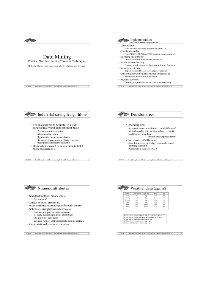
Weather data (again!)

If outlook = sunny and humidity = high then play = no If outlook = rainy and windy = true then play = no If outlook = overcast then play = yes If humidity = normal then play = yes If none of the above then play = yes … … … … … Yes False Normal Mild Rainy Yes False High Hot Overcast No True High Hot Sunny No False High Hot Sunny Play Windy Humidity Temperature Outlook … … … … … Yes False Normal Mild Rainy Yes False High Hot Overcast No True High Hot Sunny No False High Hot Sunny Play Windy Humidity Temperature Outlook … … … … … Yes False High Mild Rainy Yes False High Hot Overcast No True High Hot Sunny No False High Hot Sunny Play Windy Humidity Temperature Outlook … … … … … … … … … … No True Normal Cool Rainy … … … … … … … … … … … … … … … … … … … … … … … … … Yes False Normal Cool Rainy

1

SLIDE 2

7 Data Mining: Practical Machine Learning Tools and Techniques (Chapter 6) 07/20/06

Weather data (again!)

If outlook = sunny and humidity = high then play = no If outlook = rainy and windy = true then play = no If outlook = overcast then play = yes If humidity = normal then play = yes If none of the above then play = yes If outlook = sunny and humidity > 83 then play = no If outlook = rainy and windy = true then play = no If outlook = overcast then play = yes If humidity < 85 then play = no If none of the above then play = yes … … … … … Yes False Normal Mild Rainy Yes False High Hot Overcast No True High Hot Sunny No False High Hot Sunny Play Windy Humidity Temperature Outlook … … … … … Yes False Normal Mild Rainy Yes False High Hot Overcast No True High Hot Sunny No False High Hot Sunny Play Windy Humidity Temperature Outlook … … … … … Yes False High Mild Rainy Yes False High Hot Overcast No True High Hot Sunny No False High Hot Sunny Play Windy Humidity Temperature Outlook … … … … … … … … … … No True Normal Cool Rainy … … … … … … … … … … … … … … … … … … … … … … … … … Yes False Normal Cool Rainy … … … … … Yes False Normal Mild Rainy Yes False High Hot Overcast No True High Hot Sunny No False High Hot Sunny Play Windy Humidity Temperature Outlook … … … … … Yes False Normal Mild Rainy Yes False High Hot Overcast No True High Hot Sunny No False High Hot Sunny Play Windy Humidity Temperature Outlook … … … … … Yes False 96 70 Rainy Yes False 86 83 Overcast No True 90 80 Sunny No False 85 85 Sunny Play Windy Humidity Temperature Outlook … … … … … … … … … … No True 70 65 Rainy … … … … … … … … … … … … … … … … … … … … … … … … … Yes False 80 68 Rainy 8 Data Mining: Practical Machine Learning Tools and Techniques (Chapter 6) 07/20/06

Example

✁ Split on temperature attribute:

z E.g. temperature < 71.5: yes/4, no/2

temperature * 71.5: yes/5, no/3

z Info([4,2],[5,3])

= 6/14 info([4,2]) + 8/14 info([5,3]) = 0.939 bits

✁ Place split points halfway between values ✁ Can evaluate all split points in one pass!

64 65 68 69 70 71 72 72 75 75 80 81 83 85 Yes No Yes Yes Yes No No Yes Yes Yes No Yes Yes No 9 Data Mining: Practical Machine Learning Tools and Techniques (Chapter 6) 07/20/06

Can avoid repeated sorting

✁ Sort instances by the values of the numeric attribute

z Time complexity for sorting: O (n log n)

✁ Does this have to be repeated at each node of the

tree?

✁ No! Sort order for children can be derived from sort

• rder for parent

z Time complexity of derivation: O (n) z Drawback: need to create and store an array of sorted

indices for each numeric attribute

10 Data Mining: Practical Machine Learning Tools and Techniques (Chapter 6) 07/20/06

Binary vs multiway splits

✁ Splitting (multi-way) on a nominal attribute

exhausts all information in that attribute

z Nominal attribute is tested (at most) once on any path

in the tree

✁ Not so for binary splits on numeric attributes!

z Numeric attribute may be tested several times along a

path in the tree

✁ Disadvantage: tree is hard to read ✁ Remedy:

z pre-discretize numeric attributes, or z use multi-way splits instead of binary ones 11 Data Mining: Practical Machine Learning Tools and Techniques (Chapter 6) 07/20/06

Computing multi-way splits

✁ Simple and efficient way of generating

multi-way splits: greedy algorithm

✁ Dynamic programming can find optimum

multi-way split in O (n2) time

z imp (k, i, j ) is the impurity of the best split of

values xi … xj into k sub-intervals

z imp (k, 1, i ) =

min0<j <i imp (k–1, 1, j ) + imp (1, j+1, i )

z imp (k, 1, N ) gives us the best k-way split

✁ In practice, greedy algorithm works as well

12 Data Mining: Practical Machine Learning Tools and Techniques (Chapter 6) 07/20/06

Missing values

✁ Split instances with missing values into pieces

z A piece going down a branch receives a weight

proportional to the popularity of the branch

z weights sum to 1

✁ Info gain works with fractional instances

z use sums of weights instead of counts

✁ During classification, split the instance into

pieces in the same way

z Merge probability distribution using weights

2

SLIDE 3

13 Data Mining: Practical Machine Learning Tools and Techniques (Chapter 6) 07/20/06

Pruning

✂ Prevent overfitting to noise in the data ✂ “Prune” the decision tree ✂ Two strategies: ✄ Postpruning

take a fully-grown decision tree and discard unreliable parts

✄ Prepruning

stop growing a branch when information becomes unreliable

✂ Postpruning preferred in practice—

prepruning can “stop early”

14 Data Mining: Practical Machine Learning Tools and Techniques (Chapter 6) 07/20/06

Prepruning

✁ Based on statistical significance test

z Stop growing the tree when there is no statistically

significant association between any attribute and the class at a particular node

✁ Most popular test: chi-squared test ✁ ID3 used chi-squared test in addition to

information gain

z Only statistically significant attributes were allowed to

be selected by information gain procedure

15 Data Mining: Practical Machine Learning Tools and Techniques (Chapter 6) 07/20/06

Early stopping

• Pre-pruning may stop the growth

process prematurely: early stopping

• Classic example: XOR/Parity-problem

z No individual attribute exhibits any significant

association to the class

z Structure is only visible in fully expanded tree z Prepruning won’t expand the root node

• But: XOR-type problems rare in practice
• And: prepruning faster than postpruning

1 1 1 2 1 1 a 1 4 1 3 class b 16 Data Mining: Practical Machine Learning Tools and Techniques (Chapter 6) 07/20/06

Postpruning

✂ First, build full tree ✂ Then, prune it ✄ Fully-grown tree shows all attribute interactions ✂ Problem: some subtrees might be due to

chance effects

✂ Two pruning operations: ✄ Subtree replacement ✄ Subtree raising ✂ Possible strategies: ✄ error estimation ✄ significance testing ✄ MDL principle

17 Data Mining: Practical Machine Learning Tools and Techniques (Chapter 6) 07/20/06

Subtree replacement

• Bottom-up
• Consider replacing a tree only

after considering all its subtrees

18 Data Mining: Practical Machine Learning Tools and Techniques (Chapter 6) 07/20/06

Subtree raising

• Delete node
• Redistribute instances
• Slower than subtree

replacement (Worthwhile?)

3

SLIDE 4

19 Data Mining: Practical Machine Learning Tools and Techniques (Chapter 6) 07/20/06

Estimating error rates

✁ Prune only if it does not increase the estimated error ✁ Error on the training data is NOT a useful estimator

(would result in almost no pruning)

✁ Use hold-out set for pruning

(“reduced-error pruning”)

✁ C4.5’s method

z Derive confidence interval from training data z Use a heuristic limit, derived from this, for pruning z Standard Bernoulli-process-based method z Shaky statistical assumptions (based on training data) 20 Data Mining: Practical Machine Learning Tools and Techniques (Chapter 6) 07/20/06

C4.5’s method

✁ Error estimate for subtree is weighted sum of error

estimates for all its leaves

✁ Error estimate for a node: ✁ If c = 25% then z = 0.69 (from normal distribution) ✁ f is the error on the training data ✁ N is the number of instances covered by the leaf ✂✁☎✄ ✆✞✝✠✟ ✡ ☛ ☞ ✝☎✌✎✍ ✏ ✑☎✒ ✏ ✡ ✑ ✝✓✟ ✡ ✔ ☞ ✡ ✕ ✖ ✄✘✗✂✝✙✟ ✡ ✑ ✕

21 Data Mining: Practical Machine Learning Tools and Techniques (Chapter 6) 07/20/06

Example

f=0.33 e=0.47 f=0.5 e=0.72 f=0.33 e=0.47 f = 5/14 e = 0.46 e < 0.51 so prune! Combined using ratios 6:2:6 gives 0.51

22 Data Mining: Practical Machine Learning Tools and Techniques (Chapter 6) 07/20/06

Complexity of tree induction

✂ Assume ✄ m attributes ✄ n training instances ✄ tree depth O (log n) ✂ Building a tree

O (m n log n)

✂ Subtree replacement

O (n)

✂ Subtree raising

O (n (log n)2)

✄ Every instance may have to be redistributed at

every node between its leaf and the root

✄ Cost for redistribution (on average): O (log n) ✂ Total cost: O (m n log n) + O (n (log n)2)

23 Data Mining: Practical Machine Learning Tools and Techniques (Chapter 6) 07/20/06

From trees to rules

✂ Simple way: one rule for each leaf ✂ C4.5rules: greedily prune conditions from each

rule if this reduces its estimated error

✄ Can produce duplicate rules ✄ Check for this at the end ✂ Then ✄ look at each class in turn ✄ consider the rules for that class ✄ find a “good” subset (guided by MDL) ✂ Then rank the subsets to avoid conflicts ✂ Finally, remove rules (greedily) if this decreases

error on the training data

24 Data Mining: Practical Machine Learning Tools and Techniques (Chapter 6) 07/20/06

C4.5: choices and options

✁ C4.5rules slow for large and noisy datasets ✁ Commercial version C5.0rules uses a

different technique

z Much faster and a bit more accurate

✁ C4.5 has two parameters

z Confidence value (default 25%):

lower values incur heavier pruning

z Minimum number of instances in the two most

popular branches (default 2)

4

SLIDE 5

25 Data Mining: Practical Machine Learning Tools and Techniques (Chapter 6) 07/20/06

Discussion

✁ The most extensively studied method of

machine learning used in data mining

✁ Different criteria for attribute/test selection

rarely make a large difference

✁ Different pruning methods mainly change

the size of the resulting pruned tree

✁ C4.5 builds univariate decision trees ✁ Some TDITDT systems can build

multivariate trees (e.g. CART) TDIDT: Top-Down Induction of Decision Trees

26 Data Mining: Practical Machine Learning Tools and Techniques (Chapter 6) 07/20/06

Classification rules

✁ Common procedure: separate-and-conquer ✁ Differences:

z Search method (e.g. greedy, beam search, ...) z Test selection criteria (e.g. accuracy, ...) z Pruning method (e.g. MDL, hold-out set, ...) z Stopping criterion (e.g. minimum accuracy) z Post-processing step

✁ Also: Decision list

vs.

• ne rule set for each class

27 Data Mining: Practical Machine Learning Tools and Techniques (Chapter 6) 07/20/06

Test selection criteria

• Basic covering algorithm:

z keep adding conditions to a rule to improve its accuracy z Add the condition that improves accuracy the most

• Measure 1: p/t

z t

total instances covered by rule p number of these that are positive

z Produce rules that don’t cover negative instances,

as quickly as possible

z May produce rules with very small coverage

—special cases or noise?

• Measure 2: Information gain p (log(p/t) – log(P/T))

z P and T the positive and total numbers before the new condition was

added

z Information gain emphasizes positive rather than negative instances

• These interact with the pruning mechanism used

28 Data Mining: Practical Machine Learning Tools and Techniques (Chapter 6) 07/20/06

Missing values, numeric attributes

✁ Common treatment of missing values:

for any test, they fail

z Algorithm must either

• use other tests to separate out positive instances
• leave them uncovered until later in the process

✁ In some cases it’s better to treat “missing”

as a separate value

✁ Numeric attributes are treated just like they

are in decision trees

29 Data Mining: Practical Machine Learning Tools and Techniques (Chapter 6) 07/20/06

Pruning rules

✁ Two main strategies:

z Incremental pruning z Global pruning

✁ Other difference: pruning criterion

z Error on hold-out set (reduced-error pruning) z Statistical significance z MDL principle

✁ Also: post-pruning vs. pre-pruning

30 Data Mining: Practical Machine Learning Tools and Techniques (Chapter 6) 07/20/06

Using a pruning set

✁ For statistical validity, must evaluate

measure on data not used for training:

z This requires a growing set and a pruning set

✁ Reduced-error pruning :

build full rule set and then prune it

✁ Incremental reduced-error pruning :

simplify each rule as soon as it is built

z Can re-split data after rule has been pruned

✁ Stratification advantageous

5

SLIDE 6

31 Data Mining: Practical Machine Learning Tools and Techniques (Chapter 6) 07/20/06

Incremental reduced-error pruning

Initialize E to the instance set Until E is empty do Split E into Grow and Prune in the ratio 2:1 For each class C for which Grow contains an instance Use basic covering algorithm to create best perfect rule for C Calculate w(R): worth of rule on Prune and w(R-): worth of rule with final condition

• mitted

If w(R-) > w(R), prune rule and repeat previous step From the rules for the different classes, select the one that’s worth most (i.e. with largest w(R)) Print the rule Remove the instances covered by rule from E Continue 32 Data Mining: Practical Machine Learning Tools and Techniques (Chapter 6) 07/20/06

Measures used in IREP

✁ [p + (N – n)] / T

z (N is total number of negatives) z Counterintuitive:

• p = 2000 and n = 1000 vs. p = 1000 and n = 1

✁ Success rate p / t

z Problem: p = 1 and t = 1

• vs. p = 1000 and t = 1001

✁ (p – n) / t

z Same effect as success rate because it equals 2p/t – 1

✁ Seems hard to find a simple measure of a rule’s

worth that corresponds with intuition

33 Data Mining: Practical Machine Learning Tools and Techniques (Chapter 6) 07/20/06

Variations

✁ Generating rules for classes in order

z Start with the smallest class z Leave the largest class covered by the default rule

✁ Stopping criterion

z Stop rule production if accuracy becomes too low

✁ Rule learner RIPPER:

z Uses MDL-based stopping criterion z Employs post-processing step to modify rules

guided by MDL criterion

34 Data Mining: Practical Machine Learning Tools and Techniques (Chapter 6) 07/20/06

Using global optimization

• RIPPER: Repeated Incremental Pruning to Produce Error

Reduction (does global optimization in an efficient way)

• Classes are processed in order of increasing size
• Initial rule set for each class is generated using IREP
• An MDL-based stopping condition is used

z DL: bits needs to send examples wrt set of rules, bits

needed to send k tests, and bits for k

• Once a rule set has been produced for each class, each rule is

re-considered and two variants are produced

z One is an extended version, one is grown from scratch z Chooses among three candidates according to DL

• Final clean-up step greedily deletes rules to minimize DL

35 Data Mining: Practical Machine Learning Tools and Techniques (Chapter 6) 07/20/06

PART

✁ Avoids global optimization step used in C4.5rules

and RIPPER

✁ Generates an unrestricted decision list using basic

separate-and-conquer procedure

✁ Builds a partial decision tree to obtain a rule

z A rule is only pruned if all its implications are known z Prevents hasty generalization

✁ Uses C4.5’s procedures to build a tree

36 Data Mining: Practical Machine Learning Tools and Techniques (Chapter 6) 07/20/06

Building a partial tree

Expand-subset (S): Choose test T and use it to split set of examples into subsets Sort subsets into increasing order of average entropy while there is a subset X not yet been expanded AND all subsets expanded so far are leaves expand-subset(X) if all subsets expanded are leaves AND estimated error for subtree * estimated error for node undo expansion into subsets and make node a leaf

6

SLIDE 7

37 Data Mining: Practical Machine Learning Tools and Techniques (Chapter 6) 07/20/06

Example

38 Data Mining: Practical Machine Learning Tools and Techniques (Chapter 6) 07/20/06

Notes on PART

✁ Make leaf with maximum coverage into a rule ✁ Treat missing values just as C4.5 does

z I.e. split instance into pieces

✁ Time taken to generate a rule:

z Worst case: same as for building a pruned tree

• Occurs when data is noisy

z Best case: same as for building a single rule

• Occurs when data is noise free

39 Data Mining: Practical Machine Learning Tools and Techniques (Chapter 6) 07/20/06

Rules with exceptions

1.Given: a way of generating a single good rule 2.Then it’s easy to generate rules with exceptions 3.Select default class for top-level rule 4.Generate a good rule for one of the remaining classes 5.Apply this method recursively to the two subsets produced by the rule

(I.e. instances that are covered/not covered)

40 Data Mining: Practical Machine Learning Tools and Techniques (Chapter 6) 07/20/06

Iris data example

Exceptions are represented as Dotted paths, altern atives as solid on es. 41 Data Mining: Practical Machine Learning Tools and Techniques (Chapter 6) 07/20/06

Extending linear classification

✁ Linear classifiers can’t model nonlinear

class boundaries

✁ Simple trick:

z Map attributes into new space consisting of

combinations of attribute values

z E.g.: all products of n factors that can be

constructed from the attributes

✁ Example with two attributes and n = 3: ✂✁☎✄✝✆✟✞✠✆ ✡☞☛ ✄✍✌✟✞✠✆ ✌ ✞✠✌ ☛ ✄ ✡ ✞✠✆✎✞✏✌ ✌ ☛ ✄✒✑✓✞✠✌ ✡

42 Data Mining: Practical Machine Learning Tools and Techniques (Chapter 6) 07/20/06

Problems with this approach

✁ 1st problem: speed

z 10 attributes, and n = 5 ‰

>2000 coefficients

z Use linear regression with attribute selection z Run time is cubic in number of attributes

✁ 2nd problem: overfitting

z Number of coefficients is large relative to the

number of training instances

z Curse of dimensionality kicks in

7

SLIDE 8

43 Data Mining: Practical Machine Learning Tools and Techniques (Chapter 6) 07/20/06

Support vector machines

✁ Support vector machines are algorithms for

learning linear classifiers

✁ Resilient to overfitting because they learn a

particular linear decision boundary:

z The maximum margin hyperplane

✁ Fast in the nonlinear case

z Use a mathematical trick to avoid creating

“pseudo-attributes”

z The nonlinear space is created implicitly 44 Data Mining: Practical Machine Learning Tools and Techniques (Chapter 6) 07/20/06

The maximum margin hyperplane

• The instances closest to the maximum margin

hyperplane are called support vectors

45 Data Mining: Practical Machine Learning Tools and Techniques (Chapter 6) 07/20/06

Support vectors

• This means the hyperplane

can be written as

The support vectors define the maximum margin hyperplane

• All other instances can be deleted without changing its position and orientation
• ✁☎✄

✁ ☛ ✄ ✆ ✞ ✆ ☛ ✄ ✌ ✞ ✌ ✂✁✄✂ ☛✆☎✞✝✟✝ ✠✡✠ ☛✌☞ ☞✟✍ ✎✟✏ ✑ ✒ ✓ ✔✖✕✘✗ ✙✞✗ ✚ ✞✜✛ ✢✤✣ ✥ ✚ ✞

46 Data Mining: Practical Machine Learning Tools and Techniques (Chapter 6) 07/20/06

Finding support vectors

• Support vector: training instance for which _i > 0
• Determine _i and b ?—

A constrained quadratic optimization problem

z Off-the-shelf tools for solving these problems z However, special-purpose algorithms are faster z Example: Platt’s sequential minimal optimization

algorithm (implemented in WEKA)

• Note: all this assumes separable data!
• ✁✦✂

☛✦☎ ✝✟✝ ✠✡✠ ☛✌☞ ☞✟✍ ✎✟✏ ✑ ✒ ✓ ✔ ✕ ✗ ✙ ✗ ✚ ✞✦✛ ✢✌✣ ✥ ✚ ✞

47 Data Mining: Practical Machine Learning Tools and Techniques (Chapter 6) 07/20/06

Nonlinear SVMs

✁ “Pseudo attributes” represent attribute

combinations

✁ Overfitting not a problem because the

maximum margin hyperplane is stable

z There are usually few support vectors relative to

the size of the training set

✁ Computation time still an issue

z Each time the dot product is computed, all the

“pseudo attributes” must be included

48 Data Mining: Practical Machine Learning Tools and Techniques (Chapter 6) 07/20/06

A mathematical trick

✁ Avoid computing the “pseudo attributes” ✁ Compute the dot product before doing the

nonlinear mapping

✁ Example: ✁ Corresponds to a map into the instance space

spanned by all products of n attributes

✧ ✁✦★ ✝✪✩ ✝✟✝ ✠✡✠ ☛✌☞ ☞ ✍ ✎ ✏ ✑ ✒ ✓ ✔✬✫✭✗ ✮✯✗ ✄ ✰ ✱ ✄ ✲ ✕ ✳ ✰ ✱ ✕ ✴

8

SLIDE 9

49 Data Mining: Practical Machine Learning Tools and Techniques (Chapter 6) 07/20/06

Other kernel functions

✁ Mapping is called a “kernel function” ✁ Polynomial kernel ✁ We can use others: ✁ Only requirement: ✁ Examples: ✧ ✁✦★☎✝✆✩ ✝✟✝ ✠✡✠ ☛✌☞ ☞✟✍ ✎✟✏ ✑ ✒ ✓ ✔ ✫ ✗ ✮ ✗ ✄ ✰ ✱ ✄ ✲ ✕ ✳ ✰✱ ✕ ✴ ✂✁✄✂ ☛ ☎✜✝✟✝ ✠✡✠ ☛✌☞ ☞✟✍ ✎✟✏ ✑ ✒ ✓ ✔✬✕✭✗ ✙✯✗ ✁ ✛ ✚ ✞✦✛ ✢✌✣ ✥ ✚ ✞ ✣ ✁ ✛ ✚

• ✗

✂ ✚ ☎✄ ✣ ✁✝✆ ✛ ✚

• ✗

✣ ✥ ✆✪✛ ✚ ✞✄ ✣ ✟ ✄ ✰ ✧ ✗ ✠ ✰ ✧ ✄ ✕ ✁☎✄ ✰ ✧ ✗ ✳ ✰ ✧ ✄ ✝ ✗ ✕ ✡ ✁ ✛ ✚

• ✗

✂ ✚

• ✄

✣ ✁✝☛✌☞✎✍✪✛✎✏✒✑ ✓ ✔ ✕ ✏✖✓ ✔ ✗ ✘ ✡ ✌✚✙ ✡ ✣ ✁ ✛ ✚

• ✗

✂ ✚ ✞✄ ✣ ✁✝✛✒✜✌✢✤✣ ✛ ✥ ✚

• ✗

✥ ✚ ✞✄ ☛ ✂✄✣ *

50 Data Mining: Practical Machine Learning Tools and Techniques (Chapter 6) 07/20/06

Noise

✁ Have assumed that the data is separable (in

• riginal or transformed space)

✁ Can apply SVMs to noisy data by

introducing a “noise” parameter C

✁ C bounds the influence of any one training

instance on the decision boundary

z Corresponding constraint: 0 ) _i ) C

✁ Still a quadratic optimization problem ✁ Have to determine C by experimentation

51 Data Mining: Practical Machine Learning Tools and Techniques (Chapter 6) 07/20/06

Sparse data

✂ SVM algorithms speed up dramatically if the data is

sparse (i.e. many values are 0)

✂ Why? Because they compute lots and lots of dot

products

✂ Sparse data ‰

compute dot products very efficiently

✄ Iterate only over non-zero values ✂ SVMs can process sparse datasets with 10,000s of

attributes

52 Data Mining: Practical Machine Learning Tools and Techniques (Chapter 6) 07/20/06

Applications

✂ Machine vision: e.g face identification ✄ Outperforms alternative approaches (1.5% error) ✂ Handwritten digit recognition: USPS data ✄ Comparable to best alternative (0.8% error) ✂ Bioinformatics: e.g. prediction of protein

secondary structure

✂ Text classifiation ✂ Can modify SVM technique for numeric

prediction problems

53 Data Mining: Practical Machine Learning Tools and Techniques (Chapter 6) 07/20/06

Support vector regression

✄ Maximum margin hyperplane only applies to

classification

✄ However, idea of support vectors and kernel functions

can be used for regression

✄ Basic method same as in linear regression: want to

minimize error

z Difference A: ignore errors smaller than ¡ and use

absolute error instead of squared error

z Difference B: simultaneously aim to maximize flatness

• f function

✄ User-specified parameter ¡ defines “tube”

54 Data Mining: Practical Machine Learning Tools and Techniques (Chapter 6) 07/20/06

More on SVM regression

✄ If there are tubes that enclose all the training points,

the flattest of them is used

z Eg.: mean is used if 2¡ > range of target values

✄ Model can be written as:

z Support vectors: points on or outside tube z Dot product can be replaced by kernel function z Note: coefficients _imay be negative

✄ No tube that encloses all training points?

z Requires trade-off between error and flatness z Controlled by upper limit C on absolute value of

coefficients _i

✂✁✄✂ ☛✦☎✄✝✟✝ ✠ ✠ ☛✌☞ ☞✟✍ ✎ ✏ ✑ ✒ ✓ ✔✬✕✭✗ ✚ ✞✜✛ ✢ ✣ ✥ ✚ ✞

9

SLIDE 10

55 Data Mining: Practical Machine Learning Tools and Techniques (Chapter 6) 07/20/06

Examples

¡ = 2 ¡ = 1 ¡ = 0.5

56 Data Mining: Practical Machine Learning Tools and Techniques (Chapter 6) 07/20/06

The kernel perceptron

✄ Can use “kernel trick” to make non-linear classifier

using perceptron rule

✄ Observation: weight vector is modified by adding or

subtracting training instances

✄ Can represent weight vector using all instances that

have been misclassified:

z Can use

instead of ( where y is either -1 or +1)

✄ Now swap summation signs:

z Can be expressed as:

✄ Can replace dot product by kernel: ☎✄✗ ✄ ✗ ✞ ✗ ☎✄✗ ☎ ✄ ✙ ✛ ✖✣ ✞✂✁ ✛ ✬✣ ✗ ✞ ✗ ☎ ✄ ✙ ✛ ✖✣ ☎✄✗ ✞✂✁ ✛

• ✣

✗ ✞ ✗ ☎ ✄ ✙ ✛ ✖✣ ✚ ✞✂✁ ✛ ✭✣ ✥ ✚ ✞ ☎ ✄ ✙ ✛ ✖✣ ✁ ✛ ✚ ✞✄✁ ✛ ✖✣ ✂ ✚ ✞ ✣

57 Data Mining: Practical Machine Learning Tools and Techniques (Chapter 6) 07/20/06

Comments on kernel perceptron

✄ Finds separating hyperplane in space created by kernel

function (if it exists)

z But: doesn't find maximum-margin hyperplane

✄ Easy to implement, supports incremental learning ✄ Linear and logistic regression can also be upgraded

using the kernel trick

z But: solution is not “sparse”: every training instance

contributes to solution

✄ Perceptron can be made more stable by using all weight

vectors encountered during learning, not just last one (voted perceptron)

z Weight vectors vote on prediction (vote based on

number of successful classifications since inception)

58 Data Mining: Practical Machine Learning Tools and Techniques (Chapter 6) 07/20/06

Multilayer perceptrons

☎ Using kernels is only one way to build nonlinear

classifier based on perceptrons

☎ Can create network of perceptrons to approximate

arbitrary target concepts

☎ Multilayer perceptron is an example of an artificial

neural network

z Consists of: input layer, hidden layer(s), and

• utput layer

☎ Structure of MLP is usually found by experimentation ☎ Parameters can be found using backpropagation

59 Data Mining: Practical Machine Learning Tools and Techniques (Chapter 6) 07/20/06

Examples

60 Data Mining: Practical Machine Learning Tools and Techniques (Chapter 6) 07/20/06

Backpropagation

☎ How to learn weights given network structure?

z Cannot simply use perceptron learning rule because

we have hidden layer(s)

z Function we are trying to minimize: error z Can use a general function minimization technique

called gradient descent

✆ Need differentiable activation function: use sigmoid

function instead of threshold function

✆ Need differentiable error function: can't use zero-one

loss, but can use squared error

✝ ✛ ✜✣ ✁ ✆ ✆ ✞ ✏ ✟ ☞ ✑ ✏ ✔ ✘ ✠ ✁ ✆ ✌ ✛ ✙☛✡ ✝ ✛ ✯✣ ✣ ✌

10

SLIDE 11

61 Data Mining: Practical Machine Learning Tools and Techniques (Chapter 6) 07/20/06

The two activation functions

62 Data Mining: Practical Machine Learning Tools and Techniques (Chapter 6) 07/20/06

Gradient descent example

Function: x2+1 Derivative: 2x Learning rate: 0.1 Start value: 4

Can only find a local minimum!

63 Data Mining: Practical Machine Learning Tools and Techniques (Chapter 6) 07/20/06

Minimizing the error I

Need to find partial derivative of error

function for each parameter (i.e. weight)

✁ ✂ ✁ ✄ ✕ ✁ ✄ ✮ ✒ ✆ ✄ ✧ ✕ ✕ ✁ ☎ ✆ ✝ ✞ ✁ ✄ ✕ ✡ ✟ ✑ ✔ ✘ ✡ ✔ ✁ ✝ ✛ ✞✣ ✛✡✠ ✡ ✝ ✛ ✯✣ ✣

• ✁

☎✄✗ ✄ ✗ ✝ ✛

• ✗

✣ ✡ ✟ ✑ ✔ ✘ ✡ ☛ ✕✌☞✎✍✑✏ ✒ ✓✕✔✡✍✖✒ ✓ ✗ ✔ ✡ ✗ ✡ ☛ ✕ ✁ ✛ ✙ ✡ ✝ ✛

• ✣

✣ ✝ ✁ ✛ ✯✣ ✝ ✛

• ✗

✣

64 Data Mining: Practical Machine Learning Tools and Techniques (Chapter 6) 07/20/06

Minimizing the error II

☎ What about the weights for the connections from

the input to the hidden layer?

✡ ✗ ✡ ☛ ✕ ✗ ✁ ✡ ✗ ✡ ✔ ✡ ✔ ✡ ☛ ✕ ✗ ✁ ✛ ✙ ✡ ✝ ✛ ✯✣ ✣ ✝ ✁ ✛ ✯✣ ✡ ✔ ✡ ☛ ✕ ✗ ✂✁ ☎✄✗ ✄ ✗ ✝ ✛

• ✗

✣ ✁ ✝ ✁ ✄ ✕ ✗ ✁✙✘✛✚ ✁ ☎ ✆ ✝ ✕ ✞ ✁ ✄ ✕ ✗ ✡ ✗ ✡ ☛ ✕ ✗ ✁✄✛ ✙ ✡ ✝ ✛ ✜✣ ✣ ✝ ✁ ✛ ✞✣ ✄ ✗ ✝ ✁ ✛

• ✗

✣ ✞ ✗ ✡ ✟ ✑ ✔ ✕ ✘ ✡ ☛ ✕ ✗✜☞✢✍✣✏ ✒ ✓ ✗ ✔ ✡ ✔ ✕ ✡ ☛ ✕ ✗✡☞✎✍✑✏ ✒✤✓ ✗ ✔✦✥ ✗

65 Data Mining: Practical Machine Learning Tools and Techniques (Chapter 6) 07/20/06

Remarks

✆ Same process works for multiple hidden layers and

multiple output units (eg. for multiple classes)

✆ Can update weights after all training instances have been

processed or incrementally:

z batch learning vs. stochastic backpropagation z Weights are initialized to small random values

✆ How to avoid overfitting?

z Early stopping: use validation set to check when to stop z Weight decay: add penalty term to error function

✆ How to speed up learning?

z Momentum: re-use proportion of old weight change z Use optimization method that employs 2nd derivative 66 Data Mining: Practical Machine Learning Tools and Techniques (Chapter 6) 07/20/06

Radial basis function networks

Another type of feedforward network with

two layers (plus the input layer)

Hidden units represent points in instance

space and activation depends on distance

z To this end, distance is converted into

similarity: Gaussian activation function

✆ Width may be different for each hidden unit

z Points of equal activation form hypersphere

(or hyperellipsoid) as opposed to hyperplane

Output layer same as in MLP

11

SLIDE 12

67 Data Mining: Practical Machine Learning Tools and Techniques (Chapter 6) 07/20/06

Learning RBF networks

✆ Parameters: centers and widths of the RBFs + weights in

• utput layer

✆ Can learn two sets of parameters independently and still

get accurate models

z Eg.: clusters from k-means can be used to form basis

functions

z Linear model can be used based on fixed RBFs z Makes learning RBFs very efficient

✆ Disadvantage: no built-in attribute weighting based on

relevance

✆ RBF networks are related to RBF SVMs

68 Data Mining: Practical Machine Learning Tools and Techniques (Chapter 6) 07/20/06

Instance-based learning

☎ Practical problems of 1-NN scheme:

z Slow (but: fast tree-based approaches exist)

• Remedy: remove irrelevant data

z Noise (but: k -NN copes quite well with noise)

• Remedy: remove noisy instances

z All attributes deemed equally important

• Remedy: weight attributes (or simply select)

z Doesn’t perform explicit generalization

• Remedy: rule-based NN approach

69 Data Mining: Practical Machine Learning Tools and Techniques (Chapter 6) 07/20/06

Learning prototypes

☎ Only those instances involved in a decision

need to be stored

☎ Noisy instances should be filtered out ☎ Idea: only use prototypical examples

70 Data Mining: Practical Machine Learning Tools and Techniques (Chapter 6) 07/20/06

Speed up, combat noise

☎ IB2: save memory, speed up classification

z Work incrementally z Only incorporate misclassified instances z Problem: noisy data gets incorporated

☎ IB3: deal with noise

z Discard instances that don’t perform well z Compute confidence intervals for

• 1. Each instance’s success rate
• 2. Default accuracy of its class

z Accept/reject instances

• Accept if lower limit of 1 exceeds upper limit of 2
• Reject if upper limit of 1 is below lower limit of 2

71 Data Mining: Practical Machine Learning Tools and Techniques (Chapter 6) 07/20/06

Weight attributes

IB4: weight each attribute

(weights can be class-specific)

Weighted Euclidean distance: Update weights based on nearest neighbor ✆ Class correct: increase weight ✆ Class incorrect: decrease weight ✆ Amount of change for i th attribute depends on

|xi- yi|

• ✁✄✂✆☎

✝ ✁ ✞✟☎✡✠☞☛✌☎ ✍ ✝✏✎✒✑ ✑ ✑ ✎ ✂✌✓ ✝ ✁ ✞✔✓✕✠☞☛☞✓✖✍ ✝ ✍

72 Data Mining: Practical Machine Learning Tools and Techniques (Chapter 6) 07/20/06

Rectangular generalizations

• Nearest-neighbor rule is used outside rectangles
• Rectangles are rules! (But they can be more

conservative than “normal” rules.)

• Nested rectangles are rules with exceptions

12

SLIDE 13

73 Data Mining: Practical Machine Learning Tools and Techniques (Chapter 6) 07/20/06

Generalized exemplars

☎ Generalize instances into hyperrectangles

z Online: incrementally modify rectangles z Offline version: seek small set of rectangles that

cover the instances

☎ Important design decisions:

z Allow overlapping rectangles?

• Requires conflict resolution

z Allow nested rectangles? z Dealing with uncovered instances? 74 Data Mining: Practical Machine Learning Tools and Techniques (Chapter 6) 07/20/06

Separating generalized exemplars

Class 1 Class 2 Separation line

75 Data Mining: Practical Machine Learning Tools and Techniques (Chapter 6) 07/20/06

Generalized distance functions

Given: some transformation operations on

attributes

K*: similarity = probability of transforming

instance A into B by chance

✆ Average over all transformation paths ✆ Weight paths according their probability

(need way of measuring this)

Uniform way of dealing with different attribute

types

Easily generalized to give distance between sets of

instances

76 Data Mining: Practical Machine Learning Tools and Techniques (Chapter 6) 07/20/06

Numeric prediction

☎ Counterparts exist for all schemes previously

discussed

z Decision trees, rule learners, SVMs, etc.

☎ (Almost) all classification schemes can be applied

to regression problems using discretization

z Discretize the class into intervals z Predict weighted average of interval midpoints z Weight according to class probabilities 77 Data Mining: Practical Machine Learning Tools and Techniques (Chapter 6) 07/20/06

Regression trees

☎ Like decision trees, but:

z Splitting criterion:

minimize intra-subset variation

z Termination criterion:

std dev becomes small

z Pruning criterion:

based on numeric error measure

z Prediction:

Leaf predicts average class values of instances

☎ Piecewise constant functions ☎ Easy to interpret ☎ More sophisticated version: model trees

78 Data Mining: Practical Machine Learning Tools and Techniques (Chapter 6) 07/20/06

Model trees

☎ Build a regression tree ☎ Each leaf ‰

linear regression function

☎ Smoothing: factor in ancestor’s predictions

z Smoothing formula: z Same effect can be achieved by incorporating

ancestor models into the leaves

☎ Need linear regression function at each node ☎ At each node, use only a subset of attributes

z Those occurring in subtree z (+maybe those occurring in path to the root)

☎ Fast: tree usually uses only a small subset of

the attributes

✂✁ ✄ ✴ ☎ ✞✝✆ ✞ ✴ ✞✝✆

13

SLIDE 14

79 Data Mining: Practical Machine Learning Tools and Techniques (Chapter 6) 07/20/06

Building the tree

• Splitting: standard deviation reduction
• Termination:

z Standard deviation < 5% of its value on full training set z Too few instances remain (e.g. < 4)

Pruning:

z Heuristic estimate of absolute error of LR models: z Greedily remove terms from LR models to minimize

estimated error

z Heavy pruning: single model may replace whole subtree z Proceed bottom up: compare error of LR model at internal

node to error of subtree

✁✄✂✆☎ ✁✞✝✠✟ ✛☛✡ ✣ ✡✦☎✄✗✌☞ ✍ ✕ ✍ ☞ ✎ ✝✠✟✆✛☛✡ ✗ ✣ ✴ ✞✑✏ ✴ ✏ ✏✓✒✕✔✗✖✙✘✓✚✛✔✢✜✣✘✥✤✗✔✢✦✄✧✠★✢✩ ✪✣✫✌✘✥✤✗✘✗✚✛✚✬★✣✚

80 Data Mining: Practical Machine Learning Tools and Techniques (Chapter 6) 07/20/06

Nominal attributes

Convert nominal attributes to binary ones ✆ Sort attribute by average class value ✆ If attribute has k values,

generate k – 1 binary attributes

✭

i th is 0 if value lies within the first i , otherwise 1

Treat binary attributes as numeric Can prove: best split on one of the new attributes

is the best (binary) split on original

81 Data Mining: Practical Machine Learning Tools and Techniques (Chapter 6) 07/20/06

Missing values

Modify splitting criterion: To determine which subset an instance goes

into, use surrogate splitting

✆ Split on the attribute whose correlation with original

is greatest

✆ Problem: complex and time-consuming ✆ Simple solution: always use the class Test set: replace missing value with average ✮✰✯✆✱ ☞✳✲ ✴ ✍ ✴ ✵✷✶ ✸✠✹ ✒✠✺✌✔ ✻✆✼ ✗☛✽ ✍ ✕ ✍ ✽ ✵✞✸✬✹ ✒✬✺ ✗ ✔ ✾

82 Data Mining: Practical Machine Learning Tools and Techniques (Chapter 6) 07/20/06

Surrogate splitting based on class

Choose split point based on instances with known

values

Split point divides instances into 2 subsets ✆

L (smaller class average)

✆

R (larger)

m is the average of the two averages For an instance with a missing value: ✆

Choose L if class value < m

✆

Otherwise R

Once full tree is built, replace missing values with

averages of corresponding leaf nodes

83 Data Mining: Practical Machine Learning Tools and Techniques (Chapter 6) 07/20/06

Pseudo-code for M5'

☎ Four methods:

z Main method: MakeModelTree z Method for splitting: split z Method for pruning: prune z Method that computes error: subtreeError

☎ We’ll briefly look at each method in turn ☎ Assume that linear regression method performs

attribute subset selection based on error

84 Data Mining: Practical Machine Learning Tools and Techniques (Chapter 6) 07/20/06

MakeModelTree

MakeModelTree (instances) { SD = sd(instances) for each k-valued nominal attribute convert into k-1 synthetic binary attributes root = newNode root.instances = instances split(root) prune(root) printTree(root) }

14

SLIDE 15

85 Data Mining: Practical Machine Learning Tools and Techniques (Chapter 6) 07/20/06

split

split(node) { if sizeof(node.instances) < 4 or sd(node.instances) < 0.05*SD node.type = LEAF else node.type = INTERIOR for each attribute for all possible split positions of attribute calculate the attribute's SDR node.attribute = attribute with maximum SDR split(node.left) split(node.right) }

86 Data Mining: Practical Machine Learning Tools and Techniques (Chapter 6) 07/20/06

prune

prune(node) { if node = INTERIOR then prune(node.leftChild) prune(node.rightChild) node.model = linearRegression(node) if subtreeError(node) > error(node) then node.type = LEAF }

87 Data Mining: Practical Machine Learning Tools and Techniques (Chapter 6) 07/20/06

subtreeError

subtreeError(node) { l = node.left; r = node.right if node = INTERIOR then return (sizeof(l.instances)*subtreeError(l) + sizeof(r.instances)*subtreeError(r)) /sizeof(node.instances) else return error(node) }

88 Data Mining: Practical Machine Learning Tools and Techniques (Chapter 6) 07/20/06

Model tree for servo data

Result

• f merging

89 Data Mining: Practical Machine Learning Tools and Techniques (Chapter 6) 07/20/06

Rules from model trees

☎ PART algorithm generates classification rules by

building partial decision trees

☎ Can use the same method to build rule sets for

regression

z Use model trees instead of decision trees z Use variance instead of entropy to choose node

to expand when building partial tree

☎ Rules will have linear models on right-hand side ☎ Caveat: using smoothed trees may not be

appropriate due to separate-and-conquer strategy

90 Data Mining: Practical Machine Learning Tools and Techniques (Chapter 6) 07/20/06

Locally weighted regression

Numeric prediction that combines ✆ instance-based learning ✆ linear regression “Lazy”: ✆ computes regression function at prediction time ✆ works incrementally Weight training instances ✆ according to distance to test instance ✆ needs weighted version of linear regression Advantage: nonlinear approximation But: slow

15

SLIDE 16

91 Data Mining: Practical Machine Learning Tools and Techniques (Chapter 6) 07/20/06

Design decisions

☎ Weighting function:

z Inverse Euclidean distance z Gaussian kernel applied to Euclidean distance z Triangular kernel used the same way z etc.

☎ Smoothing parameter is used to scale the distance

function

z Multiply distance by inverse of this parameter z Possible choice: distance of k th nearest training

instance (makes it data dependent)

92 Data Mining: Practical Machine Learning Tools and Techniques (Chapter 6) 07/20/06

Discussion

• Regression trees were introduced in CART
• Quinlan proposed model tree method (M5)
• M5’: slightly improved, publicly available
• Quinlan also investigated combining instance-

based learning with M5

• CUBIST: Quinlan’s commercial rule learner for

numeric prediction

• Interesting comparison: neural nets vs. M5

93 Data Mining: Practical Machine Learning Tools and Techniques (Chapter 6) 07/20/06

Clustering: how many clusters?

How to choose k in k-means? Possibilities:

z Choose k that minimizes cross-validated squared

distance to cluster centers

z Use penalized squared distance on the training

data (eg. using an MDL criterion)

z Apply k-means recursively with k = 2 and use

stopping criterion (eg. based on MDL)

✆ Seeds for subclusters can be chosen by seeding along

direction of greatest variance in cluster (one standard deviation away in each direction from cluster center of parent cluster)

✆ Implemented in algorithm called X-means (using

Bayesian Information Criterion instead of MDL)

94 Data Mining: Practical Machine Learning Tools and Techniques (Chapter 6) 07/20/06

Incremental clustering

☎ Heuristic approach (COBWEB/CLASSIT) ☎ Form a hierarchy of clusters incrementally ☎ Start:

z tree consists of empty root node

☎ Then:

z add instances one by one z update tree appropriately at each stage z to update, find the right leaf for an instance z May involve restructuring the tree

☎ Base update decisions on category utility

95 Data Mining: Practical Machine Learning Tools and Techniques (Chapter 6) 07/20/06

Clustering weather data

N M L K J I H G F E D C B A ID True High Mild Rainy False Normal Hot Overcast True High Mild Overcast True Normal Mild Sunny False Normal Mild Rainy False Normal Cool Sunny False High Mild Sunny True Normal Cool Overcast True Normal Cool Rainy False Normal Cool Rainy False High Mild Rainy False High Hot Overcast True High Hot Sunny False High Hot Sunny Windy Humidit y Temp. Outlook

1 2 3

96 Data Mining: Practical Machine Learning Tools and Techniques (Chapter 6) 07/20/06

Clustering weather data

N M L K J I H G F E D C B A ID True High Mild Rainy False Normal Hot Overcast True High Mild Overcast True Normal Mild Sunny False Normal Mild Rainy False Normal Cool Sunny False High Mild Sunny True Normal Cool Overcast True Normal Cool Rainy False Normal Cool Rainy False High Mild Rainy False High Hot Overcast True High Hot Sunny False High Hot Sunny Windy Humidit y Temp. Outlook

4 3

Merge best host and runner- up

5

Consider splitting the best host if merging doesn’t help

16

SLIDE 17

97 Data Mining: Practical Machine Learning Tools and Techniques (Chapter 6) 07/20/06

Final hierarchy

D C B A ID False High Mild Rainy False High Hot Overcas t True High Hot Sunny False High Hot Sunny Wind y Humidit y Temp. Outlook Oops! a and b are actually very similar 98 Data Mining: Practical Machine Learning Tools and Techniques (Chapter 6) 07/20/06

Example: the iris data (subset)

99 Data Mining: Practical Machine Learning Tools and Techniques (Chapter 6) 07/20/06

Clustering with cutoff

100 Data Mining: Practical Machine Learning Tools and Techniques (Chapter 6) 07/20/06

Category utility

☎ Category utility: quadratic loss function

defined on conditional probabilities:

☎ Every instance in different category ‰

numerator becomes

maximum

number of attributes

✂✁☎✄ ✝✆ ✞ ✠✟ ✞ ✡ ✡ ✡ ☛☞✍✌✏✎ ✑✓✒✕✔ ✖ ✗✙✘ ✚✕✔ ✛ ✒✕✜ ✒✏✢ ✣ ✖ ✗✙✘ ✤ ✜ ✥✧✦ ✜ ✢ ★ ✚✏✔ ✛ ✩ ✪✫✖ ✗✙✘ ✤ ✜ ✥✕✦ ✜ ✢ ✛ ✩ ✬ ✌ ✭✠✮✰✯✍✱✲✯✴✳✶✵✸✷✺✹ ✻✺✱ ✑✽✼ ✱ ✳✙✾ ✟

101 Data Mining: Practical Machine Learning Tools and Techniques (Chapter 6) 07/20/06

Numeric attributes

☎ Assume normal distribution: ☎ Then: ☎ Thus

becomes

☎ Prespecified minimum variance

z acuity parameter

✍ ✒ ✥ ✔ ☞ ✆ ✿ ✣ ✟✲❀ ✬ ❁❃❂❃❄❃❅ ✒✗✻ ✣ ✤✲✪✫❆ ✬ ✩ ✟ ❁ ✩ ✔ ✼ ✳✧❇✸❈ ✶ ✥ ✱ ☞✽❉ ✱ ✳ ✾ ✟✏❊✍❋ ✍ ✒ ✥ ✱ ✔ ✟ ✹ ✥ ✱ ☞ ✆ ✟ ✿ ❀ ❁ ✜ ☎✁✓✄

• ✆

✞ ✠✟ ✞ ✡ ✡ ✡ ☛✏✴✌☞✎ ✑✓✒✕✔ ✖❍✗✙✘ ✚✙✔ ✛ ✒✕✜ ✒✙✢ ✣ ✖❍✗ ✘ ✤ ✜ ✥✕✦ ✜ ✢ ★ ✚☞✔ ✛ ✩ ✪✕✖❍✗ ✘ ✤ ✜ ✥✕✦✙✜ ✢ ✛ ✩ ✬ ✌ ■❑❏ ✒ ■ ✆ ✞ ■ ✟ ✞ ▲ ▲ ▲ ▼ ■ ✌ ✔✡☞ ✒ ✔ ✖ ✗✙✘ ✚ ✔ ✛❖◆ ✩ P ◗ ✒ ✜ ✣✕◆ ❘ ❙ ❚ ✪❯◆ ❘ ❙ ✬ ✌

102 Data Mining: Practical Machine Learning Tools and Techniques (Chapter 6) 07/20/06

Probability-based clustering

❱ Problems with heuristic approach:

z Division by k? z Order of examples? z Are restructuring operations sufficient? z Is result at least local minimum of category

utility?

❱ Probabilistic perspective ‰

seek the most likely clusters given the data

❱ Also: instance belongs to a particular cluster

with a certain probability

17

SLIDE 18

103 Data Mining: Practical Machine Learning Tools and Techniques (Chapter 6) 07/20/06

Finite mixtures

❱ Model data using a mixture of distributions ❱ One cluster, one distribution

z governs probabilities of attribute values in that cluster

❱ Finite mixtures : finite number of clusters ❱ Individual distributions are normal (usually) ❱ Combine distributions using cluster weights

104 Data Mining: Practical Machine Learning Tools and Techniques (Chapter 6) 07/20/06

Two-class mixture model

A 51 A 43 B 62 B 64 A 45 A 42 A 46 A 45 A 45 B 62 A 47 A 52 B 64 A 51 B 65 A 48 A 49 A 46 B 64 A 51 A 52 B 62 A 49 A 48 B 62 A 43 A 40 A 48 B 64 A 51 B 63 A 43 B 65 B 66 B 65 A 46 A 39 B 62 B 64 A 52 B 63 B 64 A 48 B 64 A 48 A 51 A 48 B 64 A 42 A 48 A 41

data model

µA= 50, mA = 5, pA= 0.6 µB= 65, mB = 2, p B= 0.4

105 Data Mining: Practical Machine Learning Tools and Techniques (Chapter 6) 07/20/06

Using the mixture model

❱ Probability that instance x belongs to cluster A:

with

❱ Probability of an instance given the clusters: ✵✸✷✺✹ ✂✁ ✄✴✾ ✑ ✖ ✗✙✘ ☎✧★ ✆☞✛ ✖ ✗✙✘ ✆✶✛ ✖ ✗✙✘ ☎✙✛ ✑✞✝ ✣ ☎ ✟ ❆✡✠ ☛ ❁✡✠ ✬ ☞✌✠ ✖ ✗✙✘ ☎✏✛ ✍✏✎ ✑✓✒✕✔✗✖✌✘✚✙ ✛ ✆ ✿ ✣ ✟✙❀ ✬ ❁❃❂❃❄❃❅ ✎✢✜ ✣ ☎✙✪✫❆❍✬ ✩ ✟ ❁ ✩ ✙ ✵ ✷✺✹ ✄✣✁ ✤✌✥✓✦★✧✢✩✫✪ ✬✮✭✫✤✯✦✱✰✌✭✸✾ ✑ ✯ ✱ ✵✸✷✺✹ ✄✞✁ ✩✲✪ ✬✳✭✫✤✯✦✱✰ ✱ ✾ ✵✸✷✺✹ ✴★✵ ✶✗✷✫✸✺✹❃✷ ✱ ✾

106 Data Mining: Practical Machine Learning Tools and Techniques (Chapter 6) 07/20/06

Learning the clusters

❱ Assume:

z we know there are k clusters

❱ Learn the clusters ‰

z determine their parameters z I.e. means and standard deviations

❱ Performance criterion:

z probability of training data given the clusters

❱ EM algorithm

z finds a local maximum of the likelihood 107 Data Mining: Practical Machine Learning Tools and Techniques (Chapter 6) 07/20/06

EM algorithm

✻ EM = Expectation-Maximization ✼ Generalize k-means to probabilistic setting ✻ Iterative procedure: ✼ E “expectation” step:

Calculate cluster probability for each instance

✼ M “maximization” step:

Estimate distribution parameters from cluster probabilities

✻ Store cluster probabilities as instance weights ✻ Stop when improvement is negligible

108 Data Mining: Practical Machine Learning Tools and Techniques (Chapter 6) 07/20/06

More on EM

❱ Estimate parameters from weighted instances ❱ Stop when log-likelihood saturates ❱ Log-likelihood: ✔ ✆ ✛✾✽ ◆ ☎ ◆ ✿ ✽ ✩ ☎ ✩ ✿✲❀ ❀ ❀ ✿ ✽✲❁ ☎ ❁ ✽ ◆ ✿ ✽ ✩ ✿✫❀ ❀ ❀ ✿ ✽✱❁ ✘ ✆ ✛ ✽ ◆ ✣ ☎ ◆ ✪✕❆❍✬ ✩ ✿ ✽ ✩ ✣ ☎ ✩ ✪✫❆❍✬ ✩ ✿✫❀ ❀ ❀ ✿ ✽ ❁ ✣ ☎ ❁ ✪✫❆ ✬ ✩ ✽ ◆ ✿ ✽ ✩ ✿✲❀ ❀ ❀ ✿ ✽✱❁ ✯ ✱ ✪ ❂★❃ ✄ ❄ ✆ ✵✸✷✺✹ ✄ ✱ ✁

• ✾

❅ ❄✮❆ ✵✸✷✺✹ ✄ ✱ ✁ ❇●✾ ✎

18

SLIDE 19

109 Data Mining: Practical Machine Learning Tools and Techniques (Chapter 6) 07/20/06

Extending the mixture model

❱ More then two distributions: easy ❱ Several attributes: easy—assuming independence! ❱ Correlated attributes: difficult

z Joint model: bivariate normal distribution

with a (symmetric) covariance matrix

z n attributes: need to estimate n + n (n+1)/2 parameters 110 Data Mining: Practical Machine Learning Tools and Techniques (Chapter 6) 07/20/06

More mixture model extensions

✻ Nominal attributes: easy if independent ✻ Correlated nominal attributes: difficult ✼

Two correlated attributes ‰ v1 v2 parameters

✻ Missing values: easy ✻ Can use other distributions than normal: ✼

“log-normal” if predetermined minimum is given

✼

“log-odds” if bounded from above and below

✼

Poisson for attributes that are integer counts

✻ Use cross-validation to estimate k !

111 Data Mining: Practical Machine Learning Tools and Techniques (Chapter 6) 07/20/06

Bayesian clustering

❱ Problem: many parameters ‰

EM overfits

❱ Bayesian approach : give every parameter a prior

probability distribution

z Incorporate prior into overall likelihood figure z Penalizes introduction of parameters

❱ Eg: Laplace estimator for nominal attributes ❱ Can also have prior on number of clusters! ❱ Implementation: NASA’s AUTOCLASS

112 Data Mining: Practical Machine Learning Tools and Techniques (Chapter 6) 07/20/06

Discussion

❱ Can interpret clusters by using supervised

learning

z post-processing step

❱ Decrease dependence between attributes?

z pre-processing step z E.g. use principal component analysis

❱ Can be used to fill in missing values ❱ Key advantage of probabilistic clustering:

z Can estimate likelihood of data z Use it to compare different models objectively 113 Data Mining: Practical Machine Learning Tools and Techniques (Chapter 6) 07/20/06

From naïve Bayes to Bayesian Networks

• Naïve Bayes assumes:

attributes conditionally independent given the class

• Doesn’t hold in practice but classification

accuracy often high

• However: sometimes performance much

worse than e.g. decision tree

• Can we eliminate the assumption?

114 Data Mining: Practical Machine Learning Tools and Techniques (Chapter 6) 07/20/06

Enter Bayesian networks

✻ Graphical models that can represent any

probability distribution

✻ Graphical representation: directed acyclic

graph, one node for each attribute

✻ Overall probability distribution factorized

into component distributions

✻ Graph’s nodes hold component

distributions (conditional distributions)

19

SLIDE 20

115 Data Mining: Practical Machine Learning Tools and Techniques (Chapter 6) 07/20/06

N e t w

• r

k f

• r

t h e w e a t h e r d a t a

116 Data Mining: Practical Machine Learning Tools and Techniques (Chapter 6) 07/20/06

N e t w

• r

k f

• r

t h e w e a t h e r d a t a

117 Data Mining: Practical Machine Learning Tools and Techniques (Chapter 6) 07/20/06

Computing the class probabilities

✻ Two steps: computing a product of

probabilities for each class and normalization

z For each class value

✻ Take all attribute values and class value ✻ Look up corresponding entries in conditional

probability distribution tables

✻ Take the product of all probabilities

z Divide the product for each class by the sum of

the products (normalization)

118 Data Mining: Practical Machine Learning Tools and Techniques (Chapter 6) 07/20/06

Why can we do this? (Part I)

✻ Single assumption: values of a node’s

parents completely determine probability distribution for current node

• Means that node/attribute is

conditionally independent of other ancestors given parents

• ✂

✁ ☎ ✄ ✆ ✞ ✝ ✠ ✟ ☎ ✡ ✞ ☛ ☞ ✠ ✆ ☎ ✌ ✍ ✡ ✏ ✎ ✒ ✑ ✓ ✝ ☎ ✔ ✕ ✎ ✗ ✖ ✘ ✙

• ✂

✁ ✏ ✄ ✆ ✞ ✝ ✠ ✟ ☎ ✡ ✞ ☛ ✚ ✞ ☞ ✠ ✔ ✒ ✡ ✍ ✆ ✂ ✑ ✛ ✎ ✗ ✖

119 Data Mining: Practical Machine Learning Tools and Techniques (Chapter 6) 07/20/06

Why can we do this? (Part II)

✜

Chain rule from probability theory:

• Because of our assumption from the previous slide:

✵✸✷ ✹ ✻ ✆ ✞ ✻ ✟ ✞ ✡ ✡ ✡ ☛ ✻✏✢✧✾ ✑✙✣ ✱ ✥ ✆ ✢ ✵✸✷✺✹ ✻ ✱ ✁ ✻ ✱ ✪ ✆ ☛ ✡ ✡ ✡ ☛ ✻ ✆ ✾ ✤✂✥✏✦ ✧ ✆ ✞ ✧ ✟ ✞ ▲ ▲ ▲ ✖ ✧ ✢✩★ ✛✫✪ ✱ ✥ ✆ ✢ ✤✂✥☎✦ ✧ ✱ ✬ ✧ ✱ ✪ ✆ ✖ ▲ ▲ ▲ ✖ ✧ ✆ ★ ✛ ✪ ✱ ✥ ✆ ✢ ✤✂✥✠✦ ✧ ✱ ✬ ✧ ✱✍✭ ✮✰✯ ✧✠✥✛✱✍✲☎✳ ✮ ★

120 Data Mining: Practical Machine Learning Tools and Techniques (Chapter 6) 07/20/06

Learning Bayes nets

✻ Basic components of algorithms for learning

Bayes nets:

z Method for evaluating the goodness of a given

network

❱ Measure based on probability of training data

given the network (or the logarithm thereof)

z Method for searching through space of possible

networks

❱ Amounts to searching through sets of edges

because nodes are fixed

20

SLIDE 21

121 Data Mining: Practical Machine Learning Tools and Techniques (Chapter 6) 07/20/06

Problem: overfitting

❱ Can’t just maximize probability of the training

data

z Because then it’s always better to add more edges (fit

the training data more closely)

❱ Need to use cross-validation or some penalty for

complexity of the network

– AIC measure: – MDL measure: – LL: log-likelihood (log of probability of data), K: number

• f free parameters, N: #instances
• Another possibility: Bayesian approach with prior

distribution over networks

✂✁☎✄ ✮✝✆✟✞ ✥✰✱ ✛ ✜✡✠☛✠✌☞ ✍ ✎✑✏✂✒ ✮✝✆✓✞ ✥✰✱ ✛✚✜✔✠✕✠✖☞✂✗ ✟✙✘ ✚✜✛ ✢

122 Data Mining: Practical Machine Learning Tools and Techniques (Chapter 6) 07/20/06

Searching for a good structure

✻ Task can be simplified: can optimize

each node separately

z Because probability of an instance is

product of individual nodes’ probabilities

z Also works for AIC and MDL criterion

because penalties just add up

✻ Can optimize node by adding or

removing edges from other nodes

✻ Must not introduce cycles!

123 Data Mining: Practical Machine Learning Tools and Techniques (Chapter 6) 07/20/06

The K2 algorithm

✻ Starts with given ordering of nodes

(attributes)

✻ Processes each node in turn ✻ Greedily tries adding edges from

previous nodes to current node

✻ Moves to next node when current node

can’t be optimized further

✻ Result depends on initial order

124 Data Mining: Practical Machine Learning Tools and Techniques (Chapter 6) 07/20/06

Some tricks

❱ Sometimes it helps to start the search with a naïve

Bayes network

❱ It can also help to ensure that every node is in

Markov blanket of class node

z Markov blanket of a node includes all parents, children,

and children’s parents of that node

z Given values for Markov blanket, node is conditionally

independent of nodes outside blanket

z I.e. node is irrelevant to classification if not in Markov

blanket of class node

125 Data Mining: Practical Machine Learning Tools and Techniques (Chapter 6) 07/20/06

Other algorithms

❱ Extending K2 to consider greedily adding or

deleting edges between any pair of nodes

z Further step: considering inverting the direction of

edges

❱ TAN (Tree Augmented Naïve Bayes):

z Starts with naïve Bayes z Considers adding second parent to each node

(apart from class node)

z Efficient algorithm exists 126 Data Mining: Practical Machine Learning Tools and Techniques (Chapter 6) 07/20/06

Likelihood vs. conditional likelihood

❱ In classification what we really want is to

maximize probability of class given other attributes

– Not probability of the instances

❱ But: no closed-form solution for probabilities in

nodes’ tables that maximize this

❱ However: can easily compute conditional

probability of data based on given network

❱ Seems to work well when used for network scoring

21

SLIDE 22

127 Data Mining: Practical Machine Learning Tools and Techniques (Chapter 6) 07/20/06

Data structures for fast learning

❱ Learning Bayes nets involves a lot of counting for

computing conditional probabilities

❱ Naïve strategy for storing counts: hash table

z Runs into memory problems very quickly

❱ More sophisticated strategy: all-dimensions (AD) tree

z Analogous to kD-tree for numeric data z Stores counts in a tree but in a clever way such that

redundancy is eliminated

z Only makes sense to use it for large datasets 128 Data Mining: Practical Machine Learning Tools and Techniques (Chapter 6) 07/20/06

AD tree example

129 Data Mining: Practical Machine Learning Tools and Techniques (Chapter 6) 07/20/06

Building an AD tree

✻ Assume each attribute in the data has been

assigned an index

✻ Then, expand node for attribute i with the

values of all attributes j > i

z Two important restrictions:

✼ Most populous expansion for each attribute is

• mitted (breaking ties arbitrarily)

✼ Expansions with counts that are zero are also

• mitted

✻ The root node is given index zero

130 Data Mining: Practical Machine Learning Tools and Techniques (Chapter 6) 07/20/06

Discussion

✻ We have assumed: discrete data, no missing

values, no new nodes

✻ Different method of using Bayes nets for

classification: Bayesian multinets

z I.e. build one network for each class and make

prediction using Bayes’ rule

✻ Different class of learning methods for

Bayes nets: testing conditional independence assertions

✻ Can also build Bayes nets for regression

tasks

22