Network Layer Understand principles behind network layer services: - - PDF document

SLIDE 1

1

Network Layer

CS 3516 – Computer Networks CS 3516 Computer Networks Chapter 4: Network Layer

Chapter goals:

• Understand principles behind network layer

services:

– network layer service models – forwarding versus routing – how a router works – routing (path selection) – dealing with scale

• Instantiation, implementation in the Internet

Chapter 4: Network Layer

• 4. 1 Introduction
• 4.2 Virtual circuit and

datagram networks

• 4.3 What’s inside a
• 4.5 Routing algorithms

– Link state – Distance Vector – Hierarchical routing

router

• 4.4 IP: Internet

Protocol

– Datagram format – IPv4 addressing – ICMP – IPv6

• 4.6 Routing in the

Internet

– RIP – OSPF – BGP

• 4.7 Broadcast and

multicast routing

Network Layer

• Transport segment from

sending to receiving host

• On sending side

encapsulates segments into datagrams

• On rcving side delivers

application transport network data link physical network data link physical network data link physical network data link physical network data link physical network data link physical t k t k

On rcving side, delivers segments to transport layer

• Network layer protocols

in every host and router

• Router examines header

fields in all IP datagrams passing through it

application transport network data link physical network data link physical network data link physical network data link physical network data link physical network data link physical network data link physical

Two Key Network-Layer Functions

• forwarding: move

packets from router’s input to appropriate router analogy:

• routing: process of

planning trip from source to destination

• utput
• routing: determine

route taken by packets from source to destination

– routing algorithms

source to destination

• forwarding: process
• f getting through

single interchange

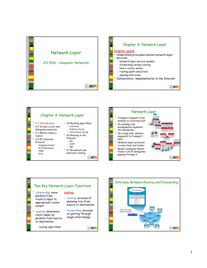
routing algorithm local forwarding table header value output link

0100 0101 0111 1001 3 2 2 1

Interplay Between Routing and Forwarding

1

2 3

0111

value in arriving packet’s header

SLIDE 2

2

Connection Setup

• 3rd important function in some network architectures:

– ATM, frame relay, X.25

• Before datagrams flow, two end hosts and intervening

routers establish virtual connection

l – routers get involved

• Network vs Transport Layer connection service:

– network: between two hosts (may also involve intervening routers in case of Virtual Circuits (VCs)) – transport: between two processes

Network Service Model

Q: What service model for “channel” transporting datagrams from sender to receiver? Example services for individual datagrams:

• Guaranteed delivery

Example services for a flow

• f datagrams:
• In order datagram
• Guaranteed delivery
• Guaranteed delivery

with less than 40 msec delay

• In-order datagram

delivery

• Guaranteed minimum

bandwidth to flow

• Restrictions on changes

in inter-packet spacing

Example Network Layer Service Models

Network Architecture Internet Service Model best effort Bandwidth none Loss no Order no Timing no Congestion feedback no (inferred via loss) Guarantees ? ATM ATM ATM ATM CBR VBR ABR UBR constant rate guaranteed rate guaranteed minimum none yes yes no no yes yes yes yes yes yes no no via loss) no congestion no congestion yes no

Chapter 4: Network Layer

• 4. 1 Introduction
• 4.2 Virtual circuit and

datagram networks

• 4.3 What’s inside a
• 4.5 Routing algorithms

– Link state – Distance Vector – Hierarchical routing

router

• 4.4 IP: Internet

Protocol

– Datagram format – IPv4 addressing – ICMP – IPv6

• 4.6 Routing in the

Internet

– RIP – OSPF – BGP

• 4.7 Broadcast and

multicast routing

Network Layer Connection and Connection-less Service

• Datagram network provides network-layer

connectionless service

• VC network provides network-layer

connection service connection service

• Analogous to the transport-layer services,

but:

– service: host-to-host – no choice: network provides one or the other – implementation: in network core

Virtual Circuits (VCs)

source-to-dest path behaves much like telephone circuit

– Performance-wise (predictable service) – Network actions along source-to-dest path

• Call setup, teardown for each call before data can flow
• Each packet carries VC identifier (not destination host

address)

• Every router on source-dest path maintains “state” for

each passing connection

• Link, router resources (bandwidth, buffers) may be

allocated to VC (dedicated resources = predictable service)

SLIDE 3

3

VC Implementation

A VC consists of:

• 1. Path from source to destination
• 2. VC numbers, one number for each link along

path 3 Entries in forwarding tables in routers along

• 3. Entries in forwarding tables in routers along

path

• Packet belonging to VC carries VC number

(rather than dest address)

• VC number can be changed on each link.

– New VC number comes from forwarding table

Forwarding Table

12 22 32

1 2 3

VC number

interface number I i i f I i VC # O i i f O i VC # (Forwarding table in northwest router) Incoming interface Incoming VC # Outgoing interface Outgoing VC # 1 12 3 22 2 63 1 18 3 7 2 17 1 97 3 87 … … … … Routers maintain connection state information!

Virtual Circuits: Signaling Protocols

• Used to setup, maintain and teardown VC
• Used in ATM, frame-relay, X.25
• Not used in today’s Internet

application transport network data link physical application transport network data link physical

• 1. Initiate call
• 2. incoming call
• 3. Accept call
• 4. Call connected
• 5. Data flow begins
• 6. Receive data

Datagram Networks

• Must do call setup at network layer
• Routers: no state about end-to-end connections

– No network-level concept of “connection”

• Packets forwarded using destination host address

– Packets between same source-dest pair may take different paths

Network Layer 4-16

application transport network data link physical application transport network data link physical

• 1. Send data
• 2. Receive data

Forwarding Table

Destination Address Range Link Interface 11001000 00010111 00010000 00000000 through 11001000 00010111 00010111 11111111

4 billion possible entries

11001000 00010111 00011000 00000000 through 1 11001000 00010111 00011000 11111111 11001000 00010111 00011001 00000000 through 2 11001000 00010111 00011111 11111111

• therwise

3

Longest Prefix Matching

Prefix Match Link Interface 11001000 00010111 00010 11001000 00010111 00011000 1 11001000 00010111 00011 2

• therwise

3

DA: 11001000 00010111 00011000 10101010

Examples

DA: 11001000 00010111 00010110 10100001

Which interface? Which interface?

SLIDE 4

4

Datagram or VC network: Why?

Internet (datagram)

• Data exchange among

computers – “Elastic” service, no strict timing req.

• “Smart” end systems

ATM (VC)

• Evolved from telephony
• Human conversation:

– strict timing, reliability requirements Smart end systems (computers) – Can adapt, perform control, error recovery – Simple inside network, complexity at “edge”

• Many link types

– Different characteristics – Uniform service difficult – need for guaranteed service

• “Dumb” end systems

– telephones – complexity inside network

Chapter 4: Network Layer

• 4. 1 Introduction
• 4.2 Virtual circuit and

datagram networks

• 4.3 What’s inside a
• 4.5 Routing algorithms

– Link state – Distance Vector – Hierarchical routing

router

• 4.4 IP: Internet

Protocol

– Datagram format – IPv4 addressing – ICMP – IPv6

• 4.6 Routing in the

Internet

– RIP – OSPF – BGP

• 4.7 Broadcast and

multicast routing

Router Architecture Overview

Two key router functions:

• Run routing algorithms/protocol (RIP, OSPF, BGP)
• Forwarding datagrams from incoming to outgoing link

Input Port Functions

Physical layer: b l l

Decentralized switching:

• Given datagram destination, lookup
• utput port using forwarding table in

input port memory

• Goal: complete input port processing at

‘line speed’

• Queuing: if datagrams arrive faster than

forwarding rate into switch fabric

bit-level reception Data link layer: e.g., Ethernet (see chapter 5)

Output Ports

• Buffering required when datagrams arrive from

fabric faster than the transmission rate

• Scheduling discipline chooses among queued

datagrams for transmission (More on queueing next slides…)

Output Port Queueing

• Buffering when arrival rate via switch exceeds
• utput line speed
• Queueing (delay) and loss due to output port

buffer overflow!

SLIDE 5

5

How Much Buffering?

• RFC 3439 rule of thumb: average buffering

equal to “typical” RTT (say 250 msec) times link capacity C (so, RTT•C)

– e g C = 10 Gps link 2 5 Gbit buffer – e.g., C = 10 Gps link 2.5 Gbit buffer

• Recent recommendation: with N flows,

buffering equal to

RTT C

.

N

Input Port Queuing

• Fabric slower than input ports combined queueing

may occur at input queues

• Head-of-the-Line (HOL) blocking: queued datagram at

front of queue prevents others in queue from moving forward

• Queueing delay and loss due to input buffer overflow!

Queueing delay and loss due to input buffer overflow!

Chapter 4: Network Layer

• 4. 1 Introduction
• 4.2 Virtual circuit and

datagram networks

• 4.3 What’s inside a
• 4.5 Routing algorithms

– Link state – Distance Vector – Hierarchical routing

router

• 4.4 IP: Internet

Protocol

– Datagram format – IPv4 addressing – ICMP – IPv6

• 4.6 Routing in the

Internet

– RIP – OSPF – BGP

• 4.7 Broadcast and

multicast routing

The Internet Network layer

Host, router network layer functions:

Routing protocols

• path selection
• RIP OSPF BGP

IP protocol

• addressing conventions
• datagram format

Transport layer: TCP, UDP N t k

forwarding table

RIP, OSPF, BGP

• packet handling conventions

ICMP protocol

• error reporting
• router “signaling”

Link layer Physical layer Network Layer

Chapter 4: Network Layer

• 4. 1 Introduction
• 4.2 Virtual circuit and

datagram networks

• 4.3 What’s inside a
• 4.5 Routing algorithms

– Link state – Distance Vector – Hierarchical routing

router

• 4.4 IP: Internet

Protocol

– Datagram format – IPv4 addressing – ICMP – IPv6

• 4.6 Routing in the

Internet

– RIP – OSPF – BGP

• 4.7 Broadcast and

multicast routing

IP Datagram Format

ver length 32 bits 16-bit identifier header checksum time to live 32 bit source IP address IP protocol version number header length (bytes) max number remaining hops (decremented at each router) for fragmentation/ reassembly total datagram length (bytes) head. len type of service “type” of data flgs fragment

• ffset

upper layer

data (variable length, typically a TCP

• r UDP segment)

upper layer protocol to deliver payload to 32 bit destination IP address Options (if any) E.g. timestamp, record route taken, specify list of routers to visit.

How much overhead with TCP?

• 20 bytes of TCP
• 20 bytes of IP
• = 40 bytes + app

layer overhead

SLIDE 6

6

IP Fragmentation & Reassembly

• Network links have MTU (max.

transfer size) - largest possible link-level frame. – different link types, different MTUs

• large IP datagram divided

(“fragmented”) within net

fragmentation: in: one large datagram

• ut: 3 smaller

datagrams

( g ) – One datagram becomes several datagrams – “Reassembled” only at final destination – IP header bits used to identify, order related fragments

reassembly

IP Fragmentation and Reassembly

ID =x

• ffset

=0 fragflag =0 length =4000 ID

• ffset

fragflag length One large datagram becomes several smaller datagrams

Example

• 4000 byte datagram
• MTU = 1500 bytes

ID =x

• ffset

=0 fragflag =1 length =1500 ID =x

• ffset

=185 fragflag =1 length =1500 ID =x

• ffset

=370 fragflag =0 length =1040 1480 bytes in data field

• ffset =

1480/8

Chapter 4: Network Layer

• 4. 1 Introduction
• 4.2 Virtual circuit and

datagram networks

• 4.3 What’s inside a
• 4.5 Routing algorithms

– Link state – Distance Vector – Hierarchical routing

router

• 4.4 IP: Internet

Protocol

– Datagram format – IPv4 addressing – ICMP – IPv6

• 4.6 Routing in the

Internet

– RIP – OSPF – BGP

• 4.7 Broadcast and

multicast routing

IP Addressing: Introduction

• IP address: 32-bit

identifier for host, router interface

• Interface: connection

between host/router and physical link

223.1.1.1 223.1.1.2 223.1.1.3 223.1.1.4 223.1.2.9 223.1.2.2 223.1.2.1 223.1.3.27

and physical link

– routers typically have multiple interfaces – hosts typically have

• ne interface

– IP addresses associated with each interface

223.1.3.2 223.1.3.1 223.1.1.1 = 11011111 00000001 00000001 00000001 223 1 1 1

Subnets

• IP address:

– subnet part (high

• rder bits)

– host part (low order bits)

• What’s a subnet ?

223.1.1.1 223.1.1.2 223.1.1.3 223.1.1.4 223.1.2.9 223.1.2.2 223.1.2.1 223.1.3.27

What s a subnet ?

– device interfaces with same subnet part of IP address – can physically reach each other without intervening router

223.1.3.2 223.1.3.1

network consisting of 3 subnets subnet

Subnets

223.1.1.0/24 223.1.2.0/24

Recipe

• To determine subnets,

detach each interface from its host or router, creating

223.1.3.0/24

, g islands of isolated networks

• Each isolated network

is called a subnet Subnet mask: /24

SLIDE 7

7

Subnets

How many?

223.1.1.1 223.1.1.3 223.1.1.4 223.1.1.2 223.1.7.0 223.1.9.2 223.1.2.2 223.1.2.1 223.1.2.6 223.1.3.2 223.1.3.1 223.1.3.27 223.1.7.1 223.1.8.0 223.1.8.1 223.1.9.1

IP addressing: CIDR

CIDR: Classless InterDomain Routing

– Subnet portion of address of arbitrary length – Address format: a.b.c.d/x, where x is # bits in subnet portion of address in subnet portion of address

11001000 00010111 00010000 00000000

subnet part host part

200.23.16.0/23

IP addresses: How to Get One?

Q: How does host get IP address?

• Hard-coded by system admin in a file

– Windows: Windows:

control-panelnetworkconfigurationTCP/IPproperties

– UNIX:

/etc/rc.config

• DHCP: Dynamic Host Configuration Protocol:

dynamically get address from as server

– “plug-and-play” – (next slide)

DHCP: Dynamic Host Configuration Protocol

Goal: allow host to dynamically obtain its IP address from network server when it joins network

– Can renew its lease on address in use – Allows reuse of addresses (only hold address while connected/”on”) – Support for mobile users who want to join network (more shortly)

• DHCP overview:

– Host broadcasts “DHCP discover” msg [optional] – DHCP server responds with “DHCP offer” msg [optional] – Host requests IP address: “DHCP request” msg – DHCP server sends address: “DHCP ack” msg

DHCP Client-Server Scenario

223.1.1.1 223.1.1.2 223.1.1.4 223.1.2.9 223.1.2.1

A

DHCP server

223.1.1.3 223.1.2.2 223.1.3.2 223.1.3.1 223.1.3.27

B E

arriving DHCP client needs address in this network

DHCP client-server scenario

DHCP server: 223.1.2.5 arriving client

DHCP discover src : 0.0.0.0, 68 dest.: 255.255.255.255,67 yiaddr: 0.0.0.0 transaction ID: 654 DHCP offer src: 223.1.2.5, 67 dest: 255.255.255.255, 68 yiaddrr: 223.1.2.4 transaction ID: 654

Network Layer

time Lifetime: 3600 secs DHCP request src: 0.0.0.0, 68 dest:: 255.255.255.255, 67 yiaddrr: 223.1.2.4 transaction ID: 655 Lifetime: 3600 secs DHCP ACK src: 223.1.2.5, 67 dest: 255.255.255.255, 68 yiaddrr: 223.1.2.4 transaction ID: 655 Lifetime: 3600 secs

SLIDE 8

8

DHCP: more than IP address

DHCP can return more than just allocated IP address on subnet:

– address of first-hop router for client n m nd IP ddr ss f DNS s v r – name and IP address of DNS sever – network mask (indicating network versus host portion of address)

DHCP: Example

• Connecting laptop needs

its IP address, addr of first-hop router, addr of DNS server use DHCP

DHCP UDP IP Eth Phy

DHCP DHCP DHCP DHCP DHCP

DHCP UDP

DHCP DHCP

• DHCP request encapsulated in

UDP, encapsulated in IP, encapsulated in 802.1 Ethernet

168 1 1 1

router (runs DHCP)

UDP IP Eth Phy

DHCP DHCP DHCP

• Ethernet frame broadcast

(dest: FFFFFFFFFFFF) on LAN, received at router running DHCP server

• Ethernet demux’ed to IP

demux’ed, UDP demux’ed to DHCP

168.1.1.1

• DCP server formulates

DHCP ACK containing client’s IP address, IP address of first-hop router for client, name & IP address of DNS server

DHCP UDP IP Eth Phy DHCP UDP

DHCP DHCP DHCP DHCP DHCP

• Encapsulation of DHCP

server, frame forwarded to client demux’ing up to

DHCP: Example

router (runs DHCP)

DHCP DHCP DHCP DHCP

UDP IP Eth Phy

to client, demux ing up to DHCP at client

• Client now knows its IP

address, name and IP address of DSN server, IP address of its first-hop router

Message type: Boot Request (1) Hardware type: Ethernet Hardware address length: 6 Hops: 0 Transaction ID: 0x6b3a11b7 Seconds elapsed: 0 Bootp flags: 0x0000 (Unicast) Client IP address: 0.0.0.0 (0.0.0.0) Your (client) IP address: 0.0.0.0 (0.0.0.0) Next server IP address: 0.0.0.0 (0.0.0.0) Relay agent IP address: 0.0.0.0 (0.0.0.0) Client MAC address: Wistron 23:68:8a (00:16:d3:23:68:8a)

DHCP: Wireshark Output (home LAN)

Message type: Boot Reply (2) Hardware type: Ethernet Hardware address length: 6 Hops: 0 Transaction ID: 0x6b3a11b7 Seconds elapsed: 0 Bootp flags: 0x0000 (Unicast) Client IP address: 192.168.1.101 (192.168.1.101) Your (client) IP address: 0.0.0.0 (0.0.0.0) Next server IP address: 192.168.1.1 (192.168.1.1) Relay agent IP address: 0.0.0.0 (0.0.0.0) Client MAC address: Wistron_23:68:8a (00:16:d3:23:68:8a) Server host name not given Boot file name not given Magic cookie: (OK) Option: (t=53,l=1) DHCP Message Type = DHCP ACK Option: (t=54,l=4) Server Identifier = 192.168.1.1 Option: (t=1 l=4) Subnet Mask = 255 255 255 0

reply request

Client MAC address: Wistron_23:68:8a (00:16:d3:23:68:8a) Server host name not given Boot file name not given Magic cookie: (OK) Option: (t=53,l=1) DHCP Message Type = DHCP Request Option: (61) Client identifier Length: 7; Value: 010016D323688A; Hardware type: Ethernet Client MAC address: Wistron_23:68:8a (00:16:d3:23:68:8a) Option: (t=50,l=4) Requested IP Address = 192.168.1.101 Option: (t=12,l=5) Host Name = "nomad" Option: (55) Parameter Request List Length: 11; Value: 010F03062C2E2F1F21F92B 1 = Subnet Mask; 15 = Domain Name 3 = Router; 6 = Domain Name Server 44 = NetBIOS over TCP/IP Name Server …… Option: (t=1,l=4) Subnet Mask = 255.255.255.0 Option: (t=3,l=4) Router = 192.168.1.1 Option: (6) Domain Name Server Length: 12; Value: 445747E2445749F244574092; IP Address: 68.87.71.226; IP Address: 68.87.73.242; IP Address: 68.87.64.146 Option: (t=15,l=20) Domain Name = "hsd1.ma.comcast.net."

IP Addressing: the Last Word...

Q: How does an ISP get block of addresses? A: ICANN: Internet Corporation for Assigned

Names and Numbers

ll t dd – allocates addresses – manages DNS – assigns domain names, resolves disputes

NAT: Network Address Translation

10.0.0.1 10.0.0.2 10.0.0.4

local network (e.g., home network) 10.0.0/24 rest of Internet

10.0.0.3 138.76.29.7

Datagrams with source or destination in this network have 10.0.0/24 address for source, destination (as usual) All datagrams leaving local network have same single source NAT IP address: 138.76.29.7, different source port numbers

SLIDE 9

9

NAT: Network Address Translation

• Motivation: local network uses just one IP

address as far as outside world is concerned:

– Range of addresses not needed from ISP: just one IP address for all devices – Can change addresses of devices in local network without notifying outside world – Can change ISP without changing addresses of devices in local network – Devices inside local net not explicitly addressable, visible by outside world (a security plus)

NAT: Network Address Translation

• Implementation: NAT router must:

– outgoing datagrams: replace (source IP address, port #)

• f every outgoing datagram to (NAT IP address, new

port #)

• (remote clients/servers will respond using (NAT IP

address new port #) as destination addr) address, new port #) as destination addr)

– remember (in NAT translation table) every (source IP address, port #) to (NAT IP address, new port #) translation pair – incoming datagrams: replace (NAT IP address, new port #) in dest fields of every incoming datagram with corresponding (source IP address, port #) stored in NAT table

NAT: Network Address Translation

10.0.0.1 S: 10.0.0.1, 3345 D: 128.119.40.186, 80

1: host 10.0.0.1 sends datagram to 128.119.40.186, 80 NAT translation table WAN side addr LAN side addr 138.76.29.7, 5001 10.0.0.1, 3345 …… …… 2: NAT router changes datagram source addr from 10.0.0.1, 3345 to 138.76.29.7, 5001, updates table

10.0.0.2 10.0.0.3

1

10.0.0.4 138.76.29.7 S: 128.119.40.186, 80 D: 10.0.0.1, 3345

4

S: 138.76.29.7, 5001 D: 128.119.40.186, 80

2

S: 128.119.40.186, 80 D: 138.76.29.7, 5001

3 3: Reply arrives

• dest. address:

138.76.29.7, 5001 4: NAT router changes datagram dest addr from 138.76.29.7, 5001 to 10.0.0.1, 3345

NAT: Network Address Translation

• 16-bit port-number field:

– ~60,000 simultaneous connections with a single LAN-side address!

• NAT is controversial:

– Routers should only process up to layer 3 – Violates “end-to-end” argument (complexity in ends)

• NAT possibility must be taken into account by

app designers, e.g., P2P applications

– Address shortage should instead be solved by IPv6

NAT Traversal Problem

• Client wants to connect to

server with address 10.0.0.1

– Server address 10.0.0.1 local to LAN (client can’t use it as destination addr) – Only one externally visible NATted address: 138.76.29.7

10.0.0.1 10.0.0.4

Client?

NATted address 138.76.29.7

• Solution 1: statically

configure NAT to forward incoming connection requests at given port to server

– e.g. (123.76.29.7, port 2500) always forwarded to 10.0.0.1 port 25000 – But must be done ahead of time!

NAT router

138.76.29.7

NAT Traversal Problem

• Solution 2: Universal Plug and

Play (UPnP) Internet Gateway Device (IGD) Protocol. Allows NATted host to:

• Learn public IP address

(138 76 29 7)

10.0.0.1 10.0.0.4

IGD Client?

(138.76.29.7)

• Add/remove port

mappings (with lease times) i.e. automate static NAT port map configuration

– Still ahead of time, but automatic

NAT router

138.76.29.7

SLIDE 10

10

NAT Traversal Problem

• Solution 3: relaying (used in Skype)

1. NATed client establishes connection to relay

• 2. External client connects to relay
• 3. Relay bridges packets between to connections

138.76.29.7

Client

10.0.0.1

NAT router

• 1. connection to

relay initiated by NATted host

• 2. connection to

relay initiated by client

• 3. relaying

established

Chapter 4: Network Layer

• 4. 1 Introduction
• 4.2 Virtual circuit and

datagram networks

• 4.3 What’s inside a
• 4.5 Routing algorithms

– Link state – Distance Vector – Hierarchical routing

router

• 4.4 IP: Internet

Protocol

– Datagram format – IPv4 addressing – ICMP – IPv6

• 4.6 Routing in the

Internet

– RIP – OSPF – BGP

• 4.7 Broadcast and

multicast routing

ICMP: Internet Control Message Protocol

• Used by hosts & routers to

communicate network-level information

– error reporting: unreachable host, network, Type Code description 0 0 echo reply (ping) 3 0 dest. network unreachable 3 1 dest host unreachable 3 2 dest protocol unreachable 3 3 dest port unreachable port, protocol – echo request/reply (used by ping)

• Network-layer “above” IP:

– ICMP msgs carried in IP datagrams

• ICMP message: type, code plus

first 8 bytes of IP datagram causing error p 3 6 dest network unknown 3 7 dest host unknown 4 0 source quench (congestion control - not used) 8 0 echo request (ping) 9 0 route advertisement 10 0 router discovery 11 0 TTL expired 12 0 bad IP header

Traceroute and ICMP

• Source sends series of

UDP segments to dest

– First has TTL =1 – Second has TTL=2, etc. – Unlikely port number

• When ICMP message

arrives, source calculates RTT

• Traceroute does this 3

times for each router

y p

• When nth datagram

arrives to nth router:

– Router discards datagram – And sends to source ICMP message (type 11, code 0) – Message includes name of router & IP address

times for each router

Stopping criterion

• UDP segment eventually

arrives at destination host

• Destination returns ICMP

“host unreachable” packet (type 3, code 3)

• When source gets this

ICMP, stops

Chapter 4: Network Layer

• 4. 1 Introduction
• 4.2 Virtual circuit and

datagram networks

• 4.3 What’s inside a
• 4.5 Routing algorithms

– Link state – Distance Vector – Hierarchical routing

router

• 4.4 IP: Internet

Protocol

– Datagram format – IPv4 addressing – ICMP – IPv6

• 4.6 Routing in the

Internet

– RIP – OSPF – BGP

• 4.7 Broadcast and

multicast routing

IPv6

• Initial motivation: 32-bit address space soon

to be completely allocated.

• Additional motivation:

– header format helps speed p ssin /f din processing/forwarding – header changes to facilitate QoS

• IPv6 datagram format:

– fixed-length 40 byte header – no fragmentation allowed

SLIDE 11

11

IPv6 Header

Priority: identify priority among datagrams in flow Flow Label: identify datagrams in same “flow” (concept of “flow” not well defined). Next header: identify upper layer protocol for data

Other Changes from IPv4

• Checksum: removed entirely to reduce

processing time at each hop

• Options: allowed, but outside of header,

indicated by “Next Header” field

• ICMPv6: new version of ICMP

– additional message types, e.g. “Packet Too Big” – multicast group management functions

• To help transition Tunneling: IPv6

carried as payload in IPv4 datagram among IPv4 routers

Chapter 4: Network Layer

• 4. 1 Introduction
• 4.2 Virtual circuit and

datagram networks

• 4.3 What’s inside a
• 4.5 Routing algorithms

– Link state – Distance Vector – Hierarchical routing

router

• 4.4 IP: Internet

Protocol

– Datagram format – IPv4 addressing – ICMP – IPv6

• 4.6 Routing in the

Internet

– RIP – OSPF – BGP

• 4.7 Broadcast and

multicast routing

routing algorithm local forwarding table header value output link

0100 0101 0111 3 2 2

Interplay between Routing, Forwarding

Network Layer 4-64

1

2 3

0111

value in arriving packet’s header

1001 1

u y

x

w v

z

Graph Abstraction

Graph: G = (N,E) N = set of routers = {u, v, w, x, y, z} E = set of links ={(u,v), (u,x), (v,x), (v,w), (x,w), (x,y), (w,y), (w,z), (y,z)} Remark: Graph abstraction is useful in other network contexts Example: P2P, where N is set of peers and E is set of TCP connections

Graph Abstraction: Costs

u y

x

w v

z 2 2 1 3 1 2 5 3 5

• c(x,x’) = cost of link (x,x’)
• e.g. c(w,z) = 5
• Cost could always be 1, or

inversely related to bandwidth,

• r inversely related to

congestion (queuing)

• Note – cost of 1 means route is

y

x 1

• Note cost of 1 means route is

number of hops (common metric) Cost of path (x1, x2, x3,…, xp) = c(x1,x2) + c(x2,x3) + … + c(xp-1,xp) Question: What’s the least-cost path between u and z ? Routing algorithm: algorithm that finds least-cost path

SLIDE 12

12

Routing Algorithm Classification

Global or decentralized information?

Global:

• All routers have complete

topology, link cost info

• “link state” algorithms

Static or dynamic?

Static:

• Routes change slowly over

time Dynamic:

• Routes change more quickly

link state algorithms Decentralized:

• Router knows physically-

connected neighbors, link costs to neighbors

• Iterative process of

computation, exchange of info with neighbors

• “distance vector” algorithms

Routes change more quickly – Periodic update – In response to link cost changes

Chapter 4: Network Layer

• 4. 1 Introduction
• 4.2 Virtual circuit and

datagram networks

• 4.3 What’s inside a
• 4.5 Routing algorithms

– Link state – Distance Vector – Hierarchical routing

router

• 4.4 IP: Internet

Protocol

– Datagram format – IPv4 addressing – ICMP – IPv6

• 4.6 Routing in the

Internet

– RIP – OSPF – BGP

• 4.7 Broadcast and

multicast routing

A Link-State Routing Algorithm

Dijkstra’s algorithm

• Network topology (groph), link costs known to all

nodes – Accomplished via “link state broadcast” – All nodes have same info

• Compute least cost paths from one node (“source”) to

all other nodes – Gives forwarding table for that node

• Can be efficient (O(nlogn), n = # nodes)

(See 4.5.1 for details and example)

Dijkstra’s Algorithm - Output Example

u w v

z

From u, resulting shortest-path tree: u y

x

w v

z 2 2 1 3 1 1 2 5 3 5

y

x

v x y w z (u,v) (u,x) (u,x) (u,x) (u,x) destination link Resulting forwarding table in u:

Link State Updates via Flooding

• Send link information (cost, connection) to neighbors
• For each incoming packet, send to every outgoing link

– Problems?

Vast numbers of duplicate packets Vast numbers of duplicate packets

• Infinite, actually, unless we stop. How?
• Hop count: decrease each hop
• Sequence number: don’t flood twice
• Selective flooding: send only in about the right

direction

Chapter 4: Network Layer

• 4. 1 Introduction
• 4.2 Virtual circuit and

datagram networks

• 4.3 What’s inside a
• 4.5 Routing algorithms

– Link state – Distance vector – Hierarchical routing

router

• 4.4 IP: Internet

Protocol

– Datagram format – IPv4 addressing – ICMP – IPv6

• 4.6 Routing in the

Internet

– RIP – OSPF – BGP

• 4.7 Broadcast and

multicast routing

SLIDE 13

13

Distance Vector Algorithm

Bellman-Ford equation Define dx(y) := cost of least-cost path from x to y Then dx(y) = min {c(x,v) + dv(y)} where min{} is taken over all neighbors v of x

v

Bellman-Ford Example

u y

x

w v

z 2 2 1 3 1 2 5 3 5 Neighbors of u: dv(z) = 5, dx(z) = 3, dw(z) = 3 du(z) = min {c(u,v) + dv(z), ( ) d ( ) B-F equation says:

y

x 1 c(u,x) + dx(z), c(u,w) + dw(z)} = min {2 + 5, 1 + 3, 5 + 3} = 4 (via x) Node that achieves minimum is next hop in shortest path (via x above) ➜ that goes in forwarding table

Distance Vector Algorithm - State

• Dx(y) = estimate of least cost from x to y
• Node x knows cost to each neighbor v:

– c(x,v)

• Node x maintains distance vector

– Dx = [Dx(y): y є N ]

• Node x also maintains its neighbors’

distance vectors

– For each neighbor v, x maintains Dv = [Dv(y): y є N ]

Distance Vector Algorithm - Idea

• From time-to-time, each node x sends its
• wn distance vector (Dx) estimate to

neighbors

– Asynchronous (next slide)

• Wh n n d x

i s n DV stim t

• When a node x receives new DV estimate

from neighbor, it updates its own DV using B-F equation:

Dx(y) ← minv{c(x,v) + Dv(y)} for each node y N

• Under most conditions estimate Dx(y)

converges to the actual least cost dx(y)

Distance Vector Algorithm - Updates

Iterative, asynchronous:

each local iteration caused by:

• Local link cost change
• DV update message from

neighbor

wait for (change in local link

cost or msg from neighbor)

Each node: Distributed:

• Each node notifies

neighbors only when its DV changes

– neighbors then notify their neighbors if necessary

recompute estimates

if DV to any dest has changed, notify neighbors

Distance Vector Algorithm - Link Cost Changes

Link cost changes:

• Node detects local link cost change
• Updates routing info, recalculates

distance vector

• If DV changes, notify neighbors

x z

1 4 50

y

1 “good news travels fast”

At time t0, Y detects the link-cost change, updates its DV, and informs its neighbors. At time t1, Z receives the update from Y and updates its table. It computes a new least cost to X and sends its neighbors its DV. At time t2, Y receives Z’s update and updates its distance table. Y’s least costs do not change and hence Y does not send any message to Z.

SLIDE 14

14

Distance Vector Algorithm - Link Cost Changes

Link cost changes:

• Good news travels fast
• Bad news travels

slowly

• Right 44 iterations

x z

1 4 50

y

60

• Right, 44 iterations

before algorithm stabilizes (see text)

• “Count to infinity”

problem!

“Poisoned” reverse:

• If Z routes through Y to

get to X :

• Z tells Y its (Z’s) distance

to X is infinite (so Y won’t route to X via Z)

• (Will not always completely

solve count to infinity problem )

Comparison of LS and DV algorithms

Message complexity

• LS: with n nodes, E links,

O(nE) msgs sent

• DV: exchange between

neighbors only

Speed of Convergence Robustness: what happens if router malfunctions?

LS:

– node can advertise incorrect link cost – each node computes only

Speed of Convergence

• LS: O(n2) algorithm requires

O(nE) msgs – may have oscillations

• DV: convergence time varies

– may be routing loops – count-to-infinity problem each node computes only its own table

• Somewhat limits damage

DV:

– DV node can advertise incorrect path cost – Each node’s table used by

• thers
• errors propagate thru

network

Chapter 4: Network Layer

• 4. 1 Introduction
• 4.2 Virtual circuit and

datagram networks

• 4.3 What’s inside a
• 4.5 Routing algorithms

– Link state – Distance Vector – Hierarchical routing

router

• 4.4 IP: Internet

Protocol

– Datagram format – IPv4 addressing – ICMP – IPv6

• 4.6 Routing in the

Internet

– RIP – OSPF – BGP

• 4.7 Broadcast and

multicast routing

Hierarchical Routing

Our routing study thus far - idealization

• all routers identical
• network “flat”
• … not true in practice

Scale: with 200 million destinations:

• Can’t store all dest’s in

routing tables!

• Routing table exchange

would swamp links!

Administrative autonomy

• internet = network of

networks

• Each network admin may

want to control routing in its

• wn network

Hierarchical Routing

• Aggregate routers into

regions, “autonomous systems” (AS)

• Routers in same AS run

same routing protocol Gateway router

• Direct link to router in

another AS g p

– “intra-AS” routing protocol – Routers in different AS can run different intra- AS routing protocol 3b 1d 3a 1c 2a AS3 AS1

AS2

1a 2c 2b 1b 3c

Interconnected ASes

• Forwarding table

d

Intra-AS Routing algorithm Inter-AS Routing algorithm

Forwarding table

Forwarding table configured by both intra- and inter-AS routing algorithm

– intra-AS sets entries for internal dests – inter-AS & intra-AS sets entries for external dests

SLIDE 15

15

Chapter 4: Network Layer

• 4. 1 Introduction
• 4.2 Virtual circuit and

datagram networks

• 4.3 What’s inside a
• 4.5 Routing algorithms

– Link state – Distance Vector – Hierarchical routing

router

• 4.4 IP: Internet

Protocol

– Datagram format – IPv4 addressing – ICMP – IPv6

• 4.6 Routing in the

Internet

– RIP – OSPF – BGP

• 4.7 Broadcast and

multicast routing

Intra-AS Routing

• Also known as Interior Gateway Protocols (IGP)
• Most common Intra-AS routing protocols:

– RIP: Routing Information Protocol – OSPF: Open Shortest Path First – IGRP: Interior Gateway Routing Protocol (Cisco proprietary)

Chapter 4: Network Layer

• 4. 1 Introduction
• 4.2 Virtual circuit and

datagram networks

• 4.3 What’s inside a
• 4.5 Routing algorithms

– Link state – Distance Vector – Hierarchical routing

router

• 4.4 IP: Internet

Protocol

– Datagram format – IPv4 addressing – ICMP – IPv6

• 4.6 Routing in the

Internet

– RIP – OSPF – BGP

• 4.7 Broadcast and

multicast routing

RIP (Routing Information Protocol)

• Distance vector algorithm
• Included in BSD-UNIX Distribution in 1982
• Distance metric: # of hops (max = 15 hops)

D

C

B A

u v w x y z destination hops u 1 v 2 w 2 x 3 y 3 z 2 From router A to subnets:

RIP Advertisements

• Distance vectors: exchanged among

neighbors every 30 sec via Response Message (also called advertisement)

• Each advertisement: list of up to 25
• Each advertisement: list of up to 25

destination subnets within AS

RIP: Example

w x y z A C D B

Destination Network Next Router Num. of hops to dest.

w A 2 y B 2 z B 7 x

• 1

…. …. ....

C Routing/Forwarding table in D

SLIDE 16

16

RIP: Example

w x y z A D B

Dest Next hops w

• 1

x

• 1

z C 4 …. … ...

Advertisement from A to D Destination Network Next Router Num. of hops to dest.

w A 2 y B 2 z B A 7 5 x

• 1

…. …. ....

C

RIP: Link Failure and Recovery

If no advertisement heard after 180 sec neighbor/link declared dead

– routes via neighbor invalidated – new advertisements sent to neighbors neighbors in turn send out new advertisements – neighbors in turn send out new advertisements (if tables changed) – link failure info quickly propagates to entire net – poison reverse used to prevent ping-pong loops (infinite distance = 16 hops)

RIP Table Processing

• RIP routing tables managed by application-level

process called route-d (d for daemon)

• Advertisements sent in UDP packets, periodically

repeated

physical link network forwarding (IP) table Transprt (UDP) routed physical link network (IP) Transprt (UDP) routed forwarding table

Chapter 4: Network Layer

• 4. 1 Introduction
• 4.2 Virtual circuit and

datagram networks

• 4.3 What’s inside a
• 4.5 Routing algorithms

– Link state – Distance Vector – Hierarchical routing

router

• 4.4 IP: Internet

Protocol

– Datagram format – IPv4 addressing – ICMP – IPv6

• 4.6 Routing in the

Internet

– RIP – OSPF – BGP

• 4.7 Broadcast and

multicast routing

OSPF (Open Shortest Path First)

• “Open” means publicly available, in this context
• Uses Link State algorithm

– LS packet dissemination – Topology map at each node – Route computation using Dijkstra’s algorithm

• OSPF advertisement carries one entry per neighbor

router

• Advertisements disseminated to entire AS (via

flooding)

– Carried in OSPF messages directly over IP (rather than TCP

• r UDP)

OSPF “Advanced” Features (not in RIP)

• security: all OSPF messages authenticated (to

prevent malicious intrusion)

• multiple same-cost paths allowed (only one path in

RIP)

• F

h li k lti l t t i f diff t

• For each link, multiple cost metrics for different

TOS (e.g., satellite link cost set “low” for best effort; high for real time)

• integrated uni- and multicast support:
• hierarchical OSPF in large domains

SLIDE 17

17

Chapter 4: Network Layer

• 4. 1 Introduction
• 4.2 Virtual circuit and

datagram networks

• 4.3 What’s inside a
• 4.5 Routing algorithms

– Link state – Distance Vector – Hierarchical routing

router

• 4.4 IP: Internet

Protocol

– Datagram format – IPv4 addressing – ICMP – IPv6

• 4.6 Routing in the

Internet

– RIP – OSPF – BGP

• 4.7 Broadcast and

multicast routing

Internet Inter-AS routing: BGP

• BGP (Border Gateway Protocol): the de

facto standard

• BGP provides each AS means to:
• 1. Obtain subnet reachability information

from nei hborin ASes from neighboring ASes

• 2. Propagate reachability information to all

AS-internal routers

• 3. Determine “good” routes to subnets based
• n reachability information and policy
• Allows subnet to advertise its existence to

rest of Internet: “I am here”

BGP Basics

• Pairs of routers (BGP peers) exchange routing info
• ver semi-permanent TCP connections: BGP sessions

– BGP sessions need not correspond to physical links.

• When AS2 advertises a prefix to AS1:

– AS2 promises it will forward datagrams towards that prefix

3b 1d 3a 1c 2a AS3 AS1

AS2

1a 2c 2b 1b 3c

eBGP session iBGP session

Distributing Reachability Info

• Using eBGP session between 3a and 1c, AS3 sends

prefix reachability info to AS1.

– 1c can then use iBGP do distribute new prefix info to all routers in AS1 – 1b can then re-advertise new reachability info to AS2

• ver 1b-to-2a eBGP session
• When router learns of new prefix, it creates entry

p y for prefix in its forwarding table.

3b 1d 3a 1c 2a AS3 AS1

AS2

1a 2c 2b 1b 3c

eBGP session iBGP session

Path Attributes and BGP Routes

• Advertised prefix includes BGP attributes.

– prefix + attributes = “route”

• Two important attributes:

– AS-PATH: contains ASs through which prefix d ti t h d AS 67 AS 17 advertisement has passed: e.g, AS 67, AS 17 – NEXT-HOP: indicates specific internal-AS router to next-hop AS (may be multiple links from current AS to next-hop-AS)

• When gateway router receives route

advertisement, uses import policy to accept/decline

BGP Route Selection

• Router may learn about more than 1 route

to some prefix. Router must select route.

• Elimination rules:

1 L l f l tt ib t li

• 1. Local preference value attribute: policy

decision

• 2. Shortest AS-PATH
• 3. Closest NEXT-HOP router: hot potato

routing

• 4. Additional criteria

SLIDE 18

18

BGP messages

• BGP messages exchanged using TCP
• BGP messages:

– OPEN: opens TCP connection to peer and authenticates sender UPDATE d ti th ( ithd – UPDATE: advertises new path (or withdraws

• ld)

– KEEPALIVE keeps connection alive in absence

• f UPDATES; also ACKs OPEN request

– NOTIFICATION: reports errors in previous msg; also used to close connection

Why Different Intra- and Inter-AS Routing?

Policy:

• Inter-AS: admin wants control over how its traffic

routed, who routes through its net

• Intra-AS: single admin, so no policy decisions needed

Scale: Scale:

• hierarchical routing saves table size, reduces update

traffic Performance:

• Intra-AS: can focus on performance
• Inter-AS: policy may dominate over performance

Chapter 4: Network Layer

• 4. 1 Introduction
• 4.2 Virtual circuit and

datagram networks

• 4.3 What’s inside a
• 4.5 Routing algorithms

– Link state – Distance Vector – Hierarchical routing

router

• 4.4 IP: Internet

Protocol

– Datagram format – IPv4 addressing – ICMP – IPv6

• 4.6 Routing in the

Internet

– RIP – OSPF – BGP

• 4.7 Broadcast and

multicast routing