
SLIDE 1
NEARLY DE SITTER GRAVITY arXiv:1905.03780 (Cotler, KJ, Maloney) see - - PowerPoint PPT Presentation
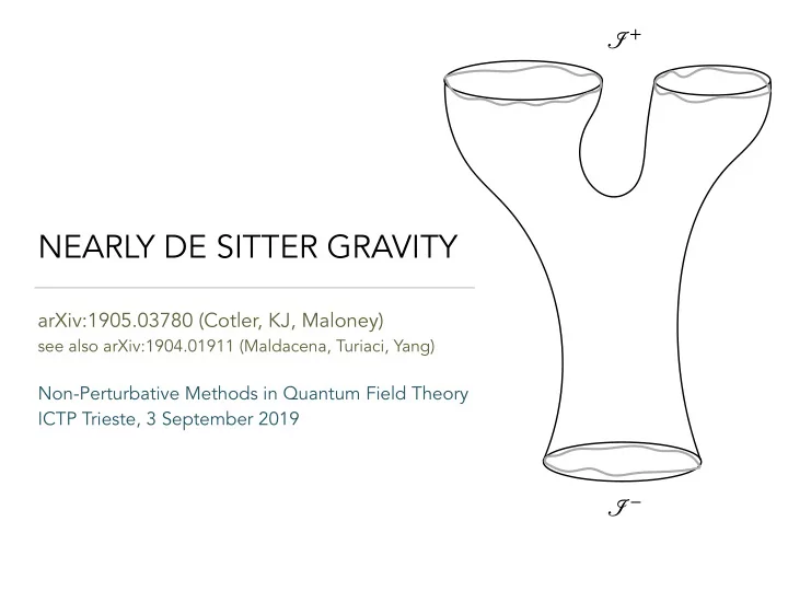
+ NEARLY DE SITTER GRAVITY arXiv:1905.03780 (Cotler, KJ, Maloney) see also arXiv:1904.01911 (Maldacena, Turiaci, Yang) Non-Perturbative Methods in Quantum Field Theory ICTP Trieste, 3 September 2019 DE SITTER HOLOGRAPHY? By now we
2
3
4
5
6
7
8
− iπ 2
9
10
11
12
14
15
{f(θ), θ} = f′′′(θ) f′(θ) − 3 2 ( f′′(θ) f′(θ) )
2
tan ( f 2 ) ∼ a tan (
f 2 ) + b
c tan (
f 2 ) + d
, ad − bc = 1
16
πi 4GβJ
17
πi 4GβJ
18
− iπ 2
19
− iπ 2
20
21
22
23
2π
+(θ)2
πiα2 4GβJ
24
25
26
− iπ 2
27
28
29
30
1 H) tr (eiβ+ 2 H) tr (e−iβ−H)⟩conn,MM,g
31
32
33
34
35
36
37