Nearest-Neighbor Methods Store all training examples Given a new - - PowerPoint PPT Presentation

About this class

k-Nearest-Neighbors Bagging Boosting

1

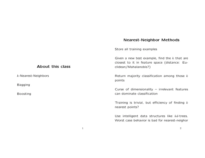
Nearest-Neighbor Methods

Store all training examples Given a new test example, find the k that are closest to it in feature space (distance: Eu- clidean/Mahalanobis?) Return majority classification among those k points Curse of dimensionality – irrelevant features can dominate classification Training is trivial, but efficiency of finding k nearest points? Use intelligent data structures like kd-trees. Worst case behavior is bad for nearest-neighor

2

search (O(l)) but much better on average (al- though distribution dependent). Initial fixed cost to building the tree Big caveat: search cost seems to scale badly with the number of dimensions in the feature space! Very simple but efective algorithm!

Bagging

Bootstrap Aggregating (Breiman, 1994) Key idea: Build t independent replicates of the training set L by sampling with replacement Train classifier on each of them Predict the majority of all these classifiers In the case of a regression problem, predict the average For decision trees: significant improvement in accuracy, but a loss in comprehensibility Works well for unstable algorithms. Intuition: unstable algorithms can change their predic- tions substantially based on small changes in the training set, which is essentially what each

3

replicate training set is doing. When you aver- age over multiple sets of training data, you’re getting a more stable predictor. Let fA be the aggregated predictor. Then fA(x) attempts to approximate ELf(x) How different are the training sets? The prob- ability that a given example is not in a given subset is (1 − 1/n)n → 1/e = 0.368 as n → ∞. Empirically, 50 replicates give all the benefit

• f bagging, often a 20% to 40% reduction in

error rate. Each trained model has higher initial variance since it is trained on a smaller training set. Bagging stable classifiers can somewhat de- grade performance What would happen with linear regression or Naive Bayes?

Boosting

Basic question: Can we take an algorithm that learns weak hypotheses that perform some- what better than chance and make it into a strong learner? Answer: yes (Freund and Schapire, various pa- pers) We’ll again build an ensemble classifier, but, unlike bagging, members of the ensemble will have different weights Bagging reduces variance (albeit slower than 1/n because the training set is replicated), but boosting reduces bias by making the hypothe- sis space more flexible

4

AdaBoost Algorithm

Given: Training examples (xi, yi), . . . , (xm, ym) A weak learning algorithm, guaranteed to make error ǫ ≤ 1

2 − γ

Maintain a weight distribution D over training

• examples. Initialize D(i) = 1/m.

Now repeat for a number of rounds T:

• 1. Train weak learner using distribution D.

This gives a weak hypothesis ht : X → {±1}. ht has error ǫt = Pr

i∼Dt

[h(xi) = yi]

5

• 2. αt ← 1

2 log 1−ǫt ǫt

• 3. Update:

D(i) ← D(i) Z e−αt if ht(xi) = yi D(i) ← D(i) Z eαt if ht(xi) = yi where Z is a normalization factor Return final hypothesis: H(x) = sgn

  T

• t=1

αtht(x)

 

Caveat: We need a weak learner that can learn even on hard weight distributions!

Training Error

First let’s bound the weight distribution: DT+1(i) = DT(i) ZT exp(−αThT(xi)yi) DT+1(i) = 1 n

T

• t=1

1 Zt exp(−αThT(xi)yi) = 1 n exp T

t=1(−αtht(xi)yi) T t=1 Zt

Now for the training error: ǫ = 1 n

• i

I[yi

• t

αtht(xi) ≤ 0] ≤ 1 n

• i

exp(−yi

• t

αtht(xi)) (because e−z ≥ 1 if z ≤ 0)

6

Substituting from above, ǫ ≤

• i

DT+1(i)

• t

Zt =

• t

Zt Finally, Zt =

• i:ht(xi)=yi

Dt(i)e−αt +

• i:ht(xi)=yi

Dt(i)eαt = e−αt(1 − ǫt) + eαt(ǫt) = 2

• ǫt(1 − ǫt)

=

• 1 − 4γ2

t

Then ǫ ≤ exp(−2

• t

γ2

t )

So, proof that we can boost weak learners that meet the requisite conditions into strong learn- ers!

Generalization and Empirical Properties

Fairly robust to overfitting. In fact, often test error keeps decreasing even after training error has converged Works well with a range of hypotheses, includ- ing decision trees, stumps, and Naive Bayes Relation to SVMs? Can think of boosting as maximizing a different margin, and of us- ing multiple weak learners to go to a high di- mensional space, instead of using a kernel like SVMs do. Computationally, boosting is easier (LP as opposed to QP)

7