Multi-fidelity Bayesian Optimisation g ( z, x ) f ( x ) Z x z X - - PowerPoint PPT Presentation

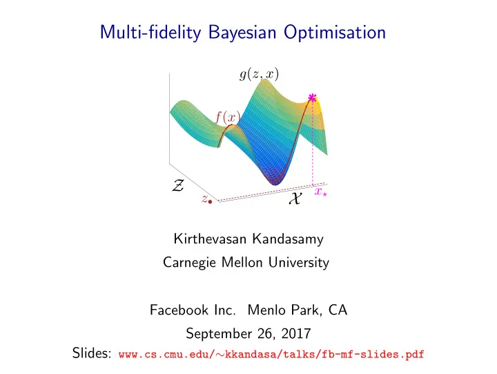
Multi-fidelity Bayesian Optimisation

x⋆

X

g(z, x) f(x) z•

Z

Kirthevasan Kandasamy Carnegie Mellon University Facebook Inc. Menlo Park, CA September 26, 2017 Slides: www.cs.cmu.edu/∼kkandasa/talks/fb-mf-slides.pdf

Slides are up on my website: www.cs.cmu.edu/∼kkandasa

Slides

Neural Network

hyper- parameters cross validation accuracy

• Train NN using given hyper-parameters
• Compute accuracy on validation set

1/30

Black-box Optimisation

Expensive Blackbox Function

1/30

Black-box Optimisation

Expensive Blackbox Function

Other Examples:

• ML estimation in astrophysics
• Pre-clinical drug discovery
• Optimal policy in autonomous driving

1/30

Black-box Optimisation

f : X → R is an expensive, black-box, noisy function, accessible

• nly via noisy evaluations.

x f(x)

2/30

Black-box Optimisation

f : X → R is an expensive, black-box, noisy function, accessible

• nly via noisy evaluations.

x f(x)

2/30

Black-box Optimisation

f : X → R is an expensive, black-box, noisy function, accessible

• nly via noisy evaluations.

Let x⋆ = argmaxx f (x).

x f(x) x∗

f(x∗)

2/30

Black-box Optimisation

f : X → R is an expensive, black-box, noisy function, accessible

• nly via noisy evaluations.

Let x⋆ = argmaxx f (x).

x f(x) x∗

f(x∗)

Simple Regret after n evaluations Sn = f (x⋆) − max

t=1,...,n f (xt).

2/30

Black-box Optimisation

f : X → R is an expensive, black-box, noisy function, accessible

• nly via noisy evaluations.

Let x⋆ = argmaxx f (x).

x f(x) x∗

f(x∗)

Cumulative Regret after n evaluations Rn =

n

• t=1
• f (x⋆) − f (xt)
• .

2/30

Black-box Optimisation

f : X → R is an expensive, black-box, noisy function, accessible

• nly via noisy evaluations.

Let x⋆ = argmaxx f (x).

x f(x) x∗

f(x∗)

Simple Regret after n evaluations Sn = f (x⋆) − max

t=1,...,n f (xt).

2/30

A walk-through Bayesian Optimisation with Gaussian Processes

◮ Gaussian Processes (GPs) ◮ GP-UCB: An algorithm for Bayesian Optimisation (BO)

3/30

Gaussian Processes (GP)

GP(µ, κ): A distribution over functions from X to R.

4/30

Gaussian Processes (GP)

GP(µ, κ): A distribution over functions from X to R. Functions with no observations

x f(x)

4/30

Gaussian Processes (GP)

GP(µ, κ): A distribution over functions from X to R. Prior GP

x f(x)

4/30

Gaussian Processes (GP)

GP(µ, κ): A distribution over functions from X to R. Observations

x f(x)

4/30

Gaussian Processes (GP)

GP(µ, κ): A distribution over functions from X to R. Posterior GP given observations

x f(x)

4/30

Gaussian Processes (GP)

GP(µ, κ): A distribution over functions from X to R. Posterior GP given observations

x f(x)

Completely characterised by mean function µ : X → R, and covariance kernel κ : X × X → R. After t observations, f (x) ∼ N( µt(x), σ2

t (x) ).

4/30

Gaussian Process Bandit (Bayesian) Optimisation

Model f ∼ GP(0, κ). Gaussian Process Upper Confidence Bound (GP-UCB)

(Srinivas et al. 2010)

x f(x)

5/30

Gaussian Process Bandit (Bayesian) Optimisation

Model f ∼ GP(0, κ). Gaussian Process Upper Confidence Bound (GP-UCB)

(Srinivas et al. 2010)

x f(x) 1) Construct posterior GP.

5/30

Gaussian Process Bandit (Bayesian) Optimisation

Model f ∼ GP(0, κ). Gaussian Process Upper Confidence Bound (GP-UCB)

(Srinivas et al. 2010)

x f(x) ϕt = µt−1 + β1/2

t

σt−1 1) Construct posterior GP. 2) ϕt = µt−1 + β1/2

t

σt−1 is a UCB.

5/30

Gaussian Process Bandit (Bayesian) Optimisation

Model f ∼ GP(0, κ). Gaussian Process Upper Confidence Bound (GP-UCB)

(Srinivas et al. 2010)

x f(x) ϕt = µt−1 + β1/2

t

σt−1

xt

1) Construct posterior GP. 2) ϕt = µt−1 + β1/2

t

σt−1 is a UCB. 3) Choose xt = argmaxx ϕt(x).

5/30

Gaussian Process Bandit (Bayesian) Optimisation

Model f ∼ GP(0, κ). Gaussian Process Upper Confidence Bound (GP-UCB)

(Srinivas et al. 2010)

x f(x) ϕt = µt−1 + β1/2

t

σt−1

xt

1) Construct posterior GP. 2) ϕt = µt−1 + β1/2

t

σt−1 is a UCB. 3) Choose xt = argmaxx ϕt(x). 4) Evaluate f at xt.

5/30

GP-UCB

(Srinivas et al. 2010)

x f(x)

6/30

GP-UCB

(Srinivas et al. 2010)

t = 1 x f(x)

6/30

GP-UCB

(Srinivas et al. 2010)

t = 2 x f(x)

6/30

GP-UCB

(Srinivas et al. 2010)

t = 3 x f(x)

6/30

GP-UCB

(Srinivas et al. 2010)

t = 4 x f(x)

6/30

GP-UCB

(Srinivas et al. 2010)

t = 5 x f(x)

6/30

GP-UCB

(Srinivas et al. 2010)

t = 6 x f(x)

6/30

GP-UCB

(Srinivas et al. 2010)

t = 7 x f(x)

6/30

GP-UCB

(Srinivas et al. 2010)

t = 11 x f(x)

6/30

GP-UCB

(Srinivas et al. 2010)

t = 25 x f(x)

6/30

GP-UCB

xt = argmax

x

µt−1(x) + β1/2

t

σt−1(x)

◮ µt−1: Exploitation ◮ σt−1: Exploration ◮ βt controls the tradeoff.

βt ≍ log t.

7/30

GP-UCB

xt = argmax

x

µt−1(x) + β1/2

t

σt−1(x)

◮ µt−1: Exploitation ◮ σt−1: Exploration ◮ βt controls the tradeoff.

βt ≍ log t. GP-UCB, κ is an SE kernel

(Srinivas et al. 2010)

w.h.p Sn = f (x⋆) − max

t=1,...,n f (xt)

• vol(X)

n

ignores constants and polylog terms.

7/30

Big picture: scaling up black-box optimisation

8/30

Big picture: scaling up black-box optimisation

◮ Optimising in high dimensional spaces

e.g.: Tuning models with several hyper-parameters Additive models for f lead to statistically and computationally tractable algorithms.

(Kandasamy et al. ICML 2015)

8/30

Big picture: scaling up black-box optimisation

◮ Optimising in high dimensional spaces

e.g.: Tuning models with several hyper-parameters Additive models for f lead to statistically and computationally tractable algorithms.

(Kandasamy et al. ICML 2015)

◮ Parallelising function evaluations

Randomised algorithms scale well to a large number of parallel workers.

(Kandasamy et al. Arxiv 2017)

8/30

Big picture: scaling up black-box optimisation

◮ Optimising in high dimensional spaces

e.g.: Tuning models with several hyper-parameters Additive models for f lead to statistically and computationally tractable algorithms.

(Kandasamy et al. ICML 2015)

◮ Parallelising function evaluations

Randomised algorithms scale well to a large number of parallel workers.

(Kandasamy et al. Arxiv 2017)

Extends beyond GPs.

8/30

This work: What if we have cheap approximations to f ?

(Kandasamy et al. NIPS 2016a&b, Kandasamy et al. ICML 2017)

9/30

This work: What if we have cheap approximations to f ?

(Kandasamy et al. NIPS 2016a&b, Kandasamy et al. ICML 2017)

• 1. Hyper-parameter tuning: Train & validate with a subset of the

data, and/or early stopping before convergence. E.g. Bandwidth (ℓ) selection in kernel density estimation.

9/30

This work: What if we have cheap approximations to f ?

(Kandasamy et al. NIPS 2016a&b, Kandasamy et al. ICML 2017)

• 1. Hyper-parameter tuning: Train & validate with a subset of the

data, and/or early stopping before convergence. E.g. Bandwidth (ℓ) selection in kernel density estimation.

• 2. Computational astrophysics: cosmological simulations and

numerical computations with less granularity.

• 3. Autonomous driving: simulation vs real world experiment.

9/30

Prior work in Multi-fidelity Methods

For specific applications,

◮ Industrial design

(Forrester et al. 2007)

◮ Hyper-parameter tuning

(Agarwal et al. 2011, Klein et al. 2015, Li et al. 2016)

◮ Active learning

(Zhang & Chaudhuri 2015)

◮ Robotics

(Cutler et al. 2014)

Multi-fidelity optimisation

(Huang et al. 2006, Forrester et al. 2007, March & Wilcox 2012, Poloczek et al. 2016)

10/30

Outline

• 1. A finite number of approximations

(Kandasamy et al. NIPS 2016b)

• Formalism, intuition and challenges
• Algorithm
• Theoretical results
• Experiments
• 2. A continuous spectrum of approximations

(Kandasamy et al. ICML 2017)

• Formalism
• Algorithm
• Theoretical results
• Experiments

11/30

Outline

• 1. A finite number of approximations

(Kandasamy et al. NIPS 2016b)

• Formalism, intuition and challenges
• Algorithm
• Theoretical results
• Experiments
• 2. A continuous spectrum of approximations

(Kandasamy et al. ICML 2017)

• Formalism
• Algorithm
• Theoretical results
• Experiments

11/30

Multi-fidelity Bandit Optimisation in 2 Fidelities (1 Approximation)

(Kandasamy et al. NIPS 2016b)

x⋆ f (2) = f ◮ Optimise f = f (2).

x⋆ = argmaxx f (2)(x).

◮ But ..

12/30

Multi-fidelity Bandit Optimisation in 2 Fidelities (1 Approximation)

(Kandasamy et al. NIPS 2016b)

x⋆ f (1) f (2) ◮ Optimise f = f (2).

x⋆ = argmaxx f (2)(x).

◮ But .. we have an approximation f (1) to f (2). ◮ f (1) costs λ(1),

f (2) costs λ(2). λ(1) < λ(2). “cost”: could be computation time, money etc.

12/30

Multi-fidelity Bandit Optimisation in 2 Fidelities (1 Approximation)

(Kandasamy et al. NIPS 2016b)

x⋆ f (1) f (2) ◮ Optimise f = f (2).

x⋆ = argmaxx f (2)(x).

◮ But .. we have an approximation f (1) to f (2). ◮ f (1) costs λ(1),

f (2) costs λ(2). λ(1) < λ(2). “cost”: could be computation time, money etc.

◮ f (1), f (2) ∼ GP(0, κ). ◮ f (2) − f (1)∞ ≤ ζ(1).

ζ(1) is known.

12/30

Multi-fidelity Bandit Optimisation in 2 Fidelities (1 Approximation)

(Kandasamy et al. NIPS 2016b)

x⋆ f (1) f (2)

At time t: Determine the point xt ∈ X and fidelity mt ∈ {1, 2} for querying.

13/30

Multi-fidelity Bandit Optimisation in 2 Fidelities (1 Approximation)

(Kandasamy et al. NIPS 2016b)

x⋆ f (1) f (2)

At time t: Determine the point xt ∈ X and fidelity mt ∈ {1, 2} for querying. End Goal: Maximise f (2). Don’t care for maximum of f (1).

13/30

Multi-fidelity Bandit Optimisation in 2 Fidelities (1 Approximation)

(Kandasamy et al. NIPS 2016b)

x⋆ f (1) f (2)

At time t: Determine the point xt ∈ X and fidelity mt ∈ {1, 2} for querying. End Goal: Maximise f (2). Don’t care for maximum of f (1). Simple Regret: S(Λ) = f (2)(x⋆) − max

t : mt=2 f (2)(xt)

Capital Λ ← amount of the resource spent. E.g. seconds or dollars.

13/30

Multi-fidelity Bandit Optimisation in 2 Fidelities (1 Approximation)

(Kandasamy et al. NIPS 2016b)

x⋆ f (1) f (2)

At time t: Determine the point xt ∈ X and fidelity mt ∈ {1, 2} for querying. End Goal: Maximise f (2). Don’t care for maximum of f (1). Simple Regret: S(Λ) = f (2)(x⋆) − max

t : mt=2 f (2)(xt)

Capital Λ ← amount of the resource spent. E.g. seconds or dollars.

No reward for querying f (1), but use cheap evaluations to guide search for x⋆ at f (2).

13/30

Challenges

x⋆ f (2) = f

13/30

Challenges

x⋆

+ζ(1) −ζ(1)

f (2)

13/30

Challenges

x⋆ f (1) f (2)

13/30

Challenges

x⋆ f (1) f (2)

◮ f (1) is not just a noisy version of f (2).

13/30

Challenges

x⋆ x(1)

⋆

f (1) f (2)

◮ f (1) is not just a noisy version of f (2). ◮ Cannot just maximise f (1).

x(1)

⋆

is suboptimal for f (2).

13/30

Challenges

x⋆ x(1)

⋆

f (1) f (2)

◮ f (1) is not just a noisy version of f (2). ◮ Cannot just maximise f (1).

x(1)

⋆

is suboptimal for f (2).

13/30

Challenges

x⋆ x(1)

⋆

f (1) f (2)

◮ f (1) is not just a noisy version of f (2). ◮ Cannot just maximise f (1).

x(1)

⋆

is suboptimal for f (2).

13/30

Challenges

x⋆ x(1)

⋆

f (1) f (2)

◮ f (1) is not just a noisy version of f (2). ◮ Cannot just maximise f (1).

x(1)

⋆

is suboptimal for f (2).

13/30

Challenges

x⋆ x(1)

⋆

f (1) f (2)

◮ f (1) is not just a noisy version of f (2). ◮ Cannot just maximise f (1).

x(1)

⋆

is suboptimal for f (2).

◮ Need to explore f (2) sufficiently well around the high valued

regions of f (1) – but at a not too large region.

13/30

Challenges

x⋆ x(1)

⋆

f(1) f(2)

◮ f (1) is not just a noisy version of f (2). ◮ Cannot just maximise f (1).

x(1)

⋆

is suboptimal for f (2).

◮ Need to explore f (2) sufficiently well around the high valued

regions of f (1) – but at a not too large region.

13/30

Challenges

x⋆ x(1)

⋆

f(1) f(2)

◮ f (1) is not just a noisy version of f (2). ◮ Cannot just maximise f (1).

x(1)

⋆

is suboptimal for f (2).

◮ Need to explore f (2) sufficiently well around the high valued

regions of f (1) – but at a not too large region.

Key Message: We will explore X using f (1) and use f (2) mostly in a promising region Xα.

13/30

MF-GP-UCB

(Kandasamy et al. NIPS 2016b)

Multi-fidelity Gaussian Process Upper Confidence Bound

x⋆ f (1) f (2)

14/30

MF-GP-UCB

(Kandasamy et al. NIPS 2016b)

Multi-fidelity Gaussian Process Upper Confidence Bound

x⋆ f (1) f (2) ◮ Construct Upper Confidence Bound ϕt for f (2).

Choose point xt = argmaxx∈X ϕt(x).

14/30

MF-GP-UCB

(Kandasamy et al. NIPS 2016b)

Multi-fidelity Gaussian Process Upper Confidence Bound

x⋆ xt t = 11 f (1) f (2) ◮ Construct Upper Confidence Bound ϕt for f (2).

Choose point xt = argmaxx∈X ϕt(x).

ϕ(1)

t (x) =

µ(1)

t−1(x) + β1/2 t

σ(1)

t−1(x) +ζ(1)

ϕ(2)

t (x) = µ(2) t−1(x) + β1/2 t

σ(2)

t−1(x)

ϕt(x) = min{ ϕ(1)

t (x), ϕ(2) t (x) } 14/30

MF-GP-UCB

(Kandasamy et al. NIPS 2016b)

Multi-fidelity Gaussian Process Upper Confidence Bound

x⋆ xt t = 11 f (1) f (2)

γ(1)

mt = 2

◮ Construct Upper Confidence Bound ϕt for f (2).

Choose point xt = argmaxx∈X ϕt(x).

ϕ(1)

t (x) =

µ(1)

t−1(x) + β1/2 t

σ(1)

t−1(x) +ζ(1)

ϕ(2)

t (x) = µ(2) t−1(x) + β1/2 t

σ(2)

t−1(x)

ϕt(x) = min{ ϕ(1)

t (x), ϕ(2) t (x) }

◮ Choose fidelity mt =

• 1

if β1/2

t

σ(1)

t−1(xt) > γ(1)

2

• therwise.

14/30

Theoretical Results for MF-GP-UCB

GP-UCB, κ is an SE kernel

(Srinivas et al. 2010)

w.h.p S(Λ) = f (2)(x⋆) − max

t : mt=2 f (2)(xt)

• vol(X)

Λ

15/30

Theoretical Results for MF-GP-UCB

GP-UCB, κ is an SE kernel

(Srinivas et al. 2010)

w.h.p S(Λ) = f (2)(x⋆) − max

t : mt=2 f (2)(xt)

• vol(X)

Λ MF-GP-UCB, κ is an SE kernel

(Kandasamy et al. NIPS 2016b)

w.h.p ∀α > 0, S(Λ)

• vol(Xα)

Λ +

• vol(X)

Λ2−α Xα = {x : f (2)(x⋆) − f (1)(x) ≤ Cαζ(1)} Good approximation (small ζ(1)) = ⇒ vol(Xα) ≪ vol(X).

15/30

MF-GP-UCB with multiple approximations

16/30

MF-GP-UCB with multiple approximations

Things work out.

16/30

Experiment: Viola & Jones Face Detection

22 Threshold values for each cascade. (d = 22) Fidelities with dataset sizes (300, 3000). (M = 2)

1000 2000 3000 4000 5000 6000 7000 8000 0.1 0.15 0.2 0.25 0.3 0.35 17/30

Experiment: Cosmological Maximum Likelihood Inference

◮ Type Ia Supernovae Data ◮ Maximum likelihood inference for 3 cosmological parameters:

◮ Hubble Constant H0 ◮ Dark Energy Fraction ΩΛ ◮ Dark Matter Fraction ΩM

◮ Likelihood: Robertson Walker metric

(Robertson 1936)

Requires numerical integration for each point in the dataset.

18/30

Experiment: Cosmological Maximum Likelihood Inference

3 cosmological parameters. (d = 3) Fidelities: integration on grids of size (102, 104, 106). (M = 3)

500 1000 1500 2000 2500 3000 3500

• 10
• 5

5 10 19/30

MF-GP-UCB Synthetic Experiment: Hartmann-3D

d = 3, M = 3

0.5 1 1.5 2 2.5 3 3.5 5 10 15 20 25 30 35 40

• Num. of Queries

Query frequencies for Hartmann-3D f (3)(x)

m=1 m=2 m=3

19/30

Outline

• 1. A finite number of approximations

(Kandasamy et al. NIPS 2016b)

• Formalism, intuition and challenges
• Algorithm
• Theoretical results
• Experiments
• 2. A continuous spectrum of approximations

(Kandasamy et al. ICML 2017)

• Formalism
• Algorithm
• Theoretical results
• Experiments

20/30

Why continuous approximations?

• Use an arbitrary amount of data?

21/30

Why continuous approximations?

• Use an arbitrary amount of data?
• Iterative algorithms: use arbitrary number of iterations?

21/30

Why continuous approximations?

• Use an arbitrary amount of data?
• Iterative algorithms: use arbitrary number of iterations?

E.g. Train an ML model with N• data and T• iterations.

• But use N < N• data and T < T• iterations to approximate

cross validation performance at (N•, T•).

21/30

Why continuous approximations?

• Use an arbitrary amount of data?
• Iterative algorithms: use arbitrary number of iterations?

E.g. Train an ML model with N• data and T• iterations.

• But use N < N• data and T < T• iterations to approximate

cross validation performance at (N•, T•). Approximations from a continuous 2D “fidelity space” (N, T).

21/30

Why continuous approximations?

• Use an arbitrary amount of data?
• Iterative algorithms: use arbitrary number of iterations?

E.g. Train an ML model with N• data and T• iterations.

• But use N < N• data and T < T• iterations to approximate

cross validation performance at (N•, T•). Approximations from a continuous 2D “fidelity space” (N, T). Scientific studies: Simulations and numerical computations at varying continuous levels of granularity.

21/30

Multi-fidelity Optimisation with Continuous Approximations

(Kandasamy et al. ICML 2017)

X Z

A fidelity space Z and domain X

Z ← all (N, T) values. X ← all hyper-parameter values.

22/30

Multi-fidelity Optimisation with Continuous Approximations

(Kandasamy et al. ICML 2017)

X

g(z, x)

Z

A fidelity space Z and domain X

Z ← all (N, T) values. X ← all hyper-parameter values.

g : Z × X → R.

g([N, T], x) ← cv accuracy when training with N data for T iterations at hyper-parameter x.

22/30

Multi-fidelity Optimisation with Continuous Approximations

(Kandasamy et al. ICML 2017)

X

g(z, x) f(x) z•

Z

A fidelity space Z and domain X

Z ← all (N, T) values. X ← all hyper-parameter values.

g : Z × X → R.

g([N, T], x) ← cv accuracy when training with N data for T iterations at hyper-parameter x.

We wish to optimise f (x) = g(z•, x) where z• ∈ Z.

z• = [N•, T•].

22/30

Multi-fidelity Optimisation with Continuous Approximations

(Kandasamy et al. ICML 2017)

x⋆

X

g(z, x) f(x) z•

Z

A fidelity space Z and domain X

Z ← all (N, T) values. X ← all hyper-parameter values.

g : Z × X → R.

g([N, T], x) ← cv accuracy when training with N data for T iterations at hyper-parameter x.

We wish to optimise f (x) = g(z•, x) where z• ∈ Z.

z• = [N•, T•].

End Goal: Find x⋆ = argmaxx f (x).

22/30

Multi-fidelity Optimisation with Continuous Approximations

(Kandasamy et al. ICML 2017)

x⋆

X

g(z, x) f(x) z•

Z

A fidelity space Z and domain X

Z ← all (N, T) values. X ← all hyper-parameter values.

g : Z × X → R.

g([N, T], x) ← cv accuracy when training with N data for T iterations at hyper-parameter x.

We wish to optimise f (x) = g(z•, x) where z• ∈ Z.

z• = [N•, T•].

End Goal: Find x⋆ = argmaxx f (x). A cost function, λ : Z → R+.

λ(z) = λ(N, T) = O(N2T).

Z z• λ(z)

22/30

Multi-fidelity Simple Regret

(Kandasamy et al. ICML 2017)

x⋆

X

g(z, x) f(x) z•

Z

Z z• λ(z) End Goal: Find x⋆ = argmaxx f (x).

23/30

Multi-fidelity Simple Regret

(Kandasamy et al. ICML 2017)

x⋆

X

g(z, x) f(x) z•

Z

Z z• λ(z) End Goal: Find x⋆ = argmaxx f (x).

Simple Regret after capital Λ:

S(Λ) = f (x⋆) − max

t: zt=z• f (xt).

Λ ← amount of a resource spent, e.g. computation time or money.

23/30

Multi-fidelity Simple Regret

(Kandasamy et al. ICML 2017)

x⋆

X

g(z, x) f(x) z•

Z

Z z• λ(z) End Goal: Find x⋆ = argmaxx f (x).

Simple Regret after capital Λ:

S(Λ) = f (x⋆) − max

t: zt=z• f (xt).

Λ ← amount of a resource spent, e.g. computation time or money. No reward for maximising low fidelities, but use cheap evaluations at z = z• to speed up search for x⋆.

23/30

BOCA: Bayesian Optimisation with Continuous Approximations

(Kandasamy et al. ICML 2017)

24/30

BOCA: Bayesian Optimisation with Continuous Approximations

(Kandasamy et al. ICML 2017)

Model g ∼ GP(0, κ) and com- pute posterior GP: mean µt−1 : Z × X → R std-dev σt−1 : Z × X → R+

24/30

BOCA: Bayesian Optimisation with Continuous Approximations

(Kandasamy et al. ICML 2017)

Model g ∼ GP(0, κ) and com- pute posterior GP: mean µt−1 : Z × X → R std-dev σt−1 : Z × X → R+ (1) xt ← maximise upper confidence bound for f (x) = g(z•, x). xt = argmax

x∈X

µt−1(z•, x) + β1/2

t

σt−1(z•, x)

24/30

BOCA: Bayesian Optimisation with Continuous Approximations

(Kandasamy et al. ICML 2017)

Model g ∼ GP(0, κ) and com- pute posterior GP: mean µt−1 : Z × X → R std-dev σt−1 : Z × X → R+ (1) xt ← maximise upper confidence bound for f (x) = g(z•, x). xt = argmax

x∈X

µt−1(z•, x) + β1/2

t

σt−1(z•, x)

24/30

BOCA: Bayesian Optimisation with Continuous Approximations

(Kandasamy et al. ICML 2017)

Model g ∼ GP(0, κ) and com- pute posterior GP: mean µt−1 : Z × X → R std-dev σt−1 : Z × X → R+ (1) xt ← maximise upper confidence bound for f (x) = g(z•, x). xt = argmax

x∈X

µt−1(z•, x) + β1/2

t

σt−1(z•, x) (2) Zt ≈ {z•} ∪

• z : σt−1(z, xt) ≥ γ(z)
• (3)

zt = argmin

z∈Zt

λ(z) (cheapest z in Zt)

24/30

BOCA: Bayesian Optimisation with Continuous Approximations

(Kandasamy et al. ICML 2017)

Model g ∼ GP(0, κ) and com- pute posterior GP: mean µt−1 : Z × X → R std-dev σt−1 : Z × X → R+ (1) xt ← maximise upper confidence bound for f (x) = g(z•, x). xt = argmax

x∈X

µt−1(z•, x) + β1/2

t

σt−1(z•, x) (2) Zt ≈ {z•} ∪

• z : σt−1(z, xt) ≥ γ(z)
• (3)

zt = argmin

z∈Zt

λ(z) (cheapest z in Zt)

24/30

BOCA: Bayesian Optimisation with Continuous Approximations

(Kandasamy et al. ICML 2017)

Model g ∼ GP(0, κ) and com- pute posterior GP: mean µt−1 : Z × X → R std-dev σt−1 : Z × X → R+ (1) xt ← maximise upper confidence bound for f (x) = g(z•, x). xt = argmax

x∈X

µt−1(z•, x) + β1/2

t

σt−1(z•, x) (2) Zt ≈ {z•} ∪

• z : σt−1(z, xt) ≥ γ(z)
• (3)

zt = argmin

z∈Zt

λ(z) (cheapest z in Zt)

24/30

BOCA: Bayesian Optimisation with Continuous Approximations

(Kandasamy et al. ICML 2017)

Model g ∼ GP(0, κ) and com- pute posterior GP: mean µt−1 : Z × X → R std-dev σt−1 : Z × X → R+ (1) xt ← maximise upper confidence bound for f (x) = g(z•, x). xt = argmax

x∈X

µt−1(z•, x) + β1/2

t

σt−1(z•, x) (2) Zt ≈ {z•} ∪

• z : σt−1(z, xt) ≥ γ(z)
• (3)

zt = argmin

z∈Zt

λ(z) (cheapest z in Zt)

24/30

BOCA: Bayesian Optimisation with Continuous Approximations

(Kandasamy et al. ICML 2017)

Model g ∼ GP(0, κ) and com- pute posterior GP: mean µt−1 : Z × X → R std-dev σt−1 : Z × X → R+ (1) xt ← maximise upper confidence bound for f (x) = g(z•, x). xt = argmax

x∈X

µt−1(z•, x) + β1/2

t

σt−1(z•, x) (2) Zt ≈ {z•} ∪

• z : σt−1(z, xt) ≥ γ(z) =

λ(z) λ(z•) q ξ(z)

• (3)

zt = argmin

z∈Zt

λ(z) (cheapest z in Zt)

24/30

Theoretical Results for BOCA

g ∼ GP(0, κ), κ : (Z × X)2 → R. κ([z, x], [z′, x′]) = κX (x, x′) · κZ(z, z′)

25/30

Theoretical Results for BOCA

g ∼ GP(0, κ), κ : (Z × X)2 → R. κ([z, x], [z′, x′]) = κX (x, x′) · κZ(z, z′)

x⋆

X

g(z, x) f(x) z•

Z “good”

x⋆ g(z, x)

X

f(x) z•

Z “bad”

25/30

Theoretical Results for BOCA

g ∼ GP(0, κ), κ : (Z × X)2 → R. κ([z, x], [z′, x′]) = κX (x, x′) · κZ(z, z′)

x⋆

X

g(z, x) f(x) z•

Z “good” large hZ

x⋆ g(z, x)

X

f(x) z•

Z “bad” small hZ E.g.: If κZ is an SE kernel, bandwidth hZ controls smoothness.

25/30

Theoretical Results for BOCA

GP-UCB κX is an SE kernel,

(Srinivas et al. 2010)

w.h.p S(Λ)

• vol(X)

Λ

26/30

Theoretical Results for BOCA

GP-UCB κX is an SE kernel,

(Srinivas et al. 2010)

w.h.p S(Λ)

• vol(X)

Λ BOCA κX , κZ are SE kernels,

(Kandasamy et al. ICML 2017)

w.h.p ∀α > 0, S(Λ)

• vol(Xα)

Λ +

• vol(X)

Λ2−α Xα =

• x; f (x⋆) − f (x) Cα

1 hZ

• 26/30

Theoretical Results for BOCA

GP-UCB κX is an SE kernel,

(Srinivas et al. 2010)

w.h.p S(Λ)

• vol(X)

Λ BOCA κX , κZ are SE kernels,

(Kandasamy et al. ICML 2017)

w.h.p ∀α > 0, S(Λ)

• vol(Xα)

Λ +

• vol(X)

Λ2−α Xα =

• x; f (x⋆) − f (x) Cα

1 hZ

• If hZ is large (good approximations), vol(Xα) ≪ vol(X),

and BOCA is much better than GP-UCB.

26/30

Experiment: SVM with 20 News Groups

Tune two hyper-parameters for the SVM. Dataset has N• = 15K data and use T• = 100 iterations. But can choose N ∈ [5K, 15K] or T ∈ [20, 100]

(2D fidelity space).

0.89 0.895 0.9 0.905 0.91 0.915 500 1000 1500 2000

More synthetic & real experiments in the paper.

27/30

Open Questions, Challenges & Take-aways

◮ If you know the relationship between the approximations

(fidelities), you should use it. Estimating it from data on the fly is not impossible, but difficult.

28/30

Open Questions, Challenges & Take-aways

◮ If you know the relationship between the approximations

(fidelities), you should use it. Estimating it from data on the fly is not impossible, but difficult.

◮ There might be better/different models for the

approximations that might suit your problem.

• E.g. approximations that are good in certain regions but bad

in other regions.

28/30

Summary

Multi-fidelity K-armed bandits

(Kandasamy et al. NIPS 2016a)

◮ An algorithm MF-UCB and an upper bound on the regret. ◮ An almost matching lower bound.

29/30

Summary

Multi-fidelity K-armed bandits

(Kandasamy et al. NIPS 2016a)

◮ An algorithm MF-UCB and an upper bound on the regret. ◮ An almost matching lower bound.

Key takeaways

(Kandasamy et al. NIPS 2016a, Kandasamy et al. NIPS 2016b, Kandasamy et al. ICML 2017)

◮ Upper confidence bound strategy ◮ Choose higher fidelity only after controlling uncertainty at

lower fidelities.

◮ Explore the entire space using cheap low fidelities and reserve

expensive higher fidelities for promising candidates.

◮ Theoretically/empirically outperforms strategies which ignore

the approximations.

29/30

Jeff Schneider Barnabas Poczos Junier Oliva Gautam Dasarathy

Thank you.

Code for MF-GP-UCB: github.com/kirthevasank/mf-gp-ucb Slides: www.cs.cmu.edu/∼kkandasa/talks/fb-mf-slides.pdf

30/30

MF-GP-UCB

(Kandasamy et al. NIPS 2016b)

x⋆ f (1) f (2)

MF-GP-UCB

(Kandasamy et al. NIPS 2016b)

x⋆ f (1) f (2)

MF-GP-UCB

(Kandasamy et al. NIPS 2016b)

x⋆ f (1) f (2)

µ(1)

t−1 + β1/2 t

σ(1)

t−1

t = 6

MF-GP-UCB

(Kandasamy et al. NIPS 2016b)

x⋆ f (1) f (2)

ϕ(1)

t

= µ(1)

t−1 + β1/2 t

σ(1)

t−1 + ζ(1)

t = 6

MF-GP-UCB

(Kandasamy et al. NIPS 2016b)

x⋆ f (1) f (2) ϕ(1)

t

ϕ(2)

t

t = 6

MF-GP-UCB

(Kandasamy et al. NIPS 2016b)

x⋆ f (1) f (2) ϕ(1)

t

ϕ(2)

t

ϕt t = 6

MF-GP-UCB

(Kandasamy et al. NIPS 2016b)

x⋆ xt t = 6 ϕ(1)

t

ϕ(2)

t

ϕt f (1) f (2)

MF-GP-UCB

(Kandasamy et al. NIPS 2016b)

x⋆ xt t = 6 ϕ(1)

t

ϕ(2)

t

ϕt f (1) f (2)

β1/2

t

σ(1)

t−1(x)

γ(1)

mt = 1

MF-GP-UCB

(Kandasamy et al. NIPS 2016b)

x⋆ xt t = 10 f (1) f (2)

γ(1)

mt = 2

MF-GP-UCB

(Kandasamy et al. NIPS 2016b)

x⋆ xt t = 11 f (1) f (2)

γ(1)

mt = 2

MF-GP-UCB

(Kandasamy et al. NIPS 2016b)

x⋆ xt t = 14 f (1) f (2)

γ(1)

mt = 2