Motivation Garbage-in, garbage-out Cannot get good mining results - PDF document

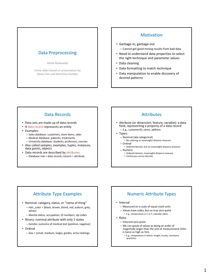
Motivation • Garbage-in, garbage-out – Cannot get good mining results from bad data Data Preprocessing • Need to understand data properties to select the right technique and parameter values • Data cleaning Mirek Riedewald • Data formatting to match technique Some slides based on presentation by • Data manipulation to enable discovery of Jiawei Han and Micheline Kamber desired patterns 2 Data Records Attributes • Data sets are made up of data records • Attribute (or dimension, feature, variable): a data field, representing a property of a data record • A data record represents an entity – E.g., customerID, name, address • Examples: • Types: – Sales database: customers, store items, sales – Nominal (aka categorical) – Medical database: patients, treatments • No ordering or meaningful distance measure – University database: students, professors, courses – Ordinal • Also called samples, examples, tuples, instances, • Ordered domain, but no meaningful distance measure data points, objects – Numeric • Data records are described by attributes • Ordered domain, meaningful distance measure – Database row = data record; column = attribute • Continuous versus discrete 3 4 Attribute Type Examples Numeric Attribute Types • Interval • Nominal: category, status, or “name of thing” – Measured on a scale of equal-sized units – Hair_color = {black, brown, blond, red, auburn, grey, – Values have order, but no true zero-point white} • E.g., temperature in C or F, calendar dates – Marital status, occupation, ID numbers, zip codes • Ratio • Binary: nominal attribute with only 2 states – Inherent zero-point – Gender, outcome of medical test (positive, negative) – We can speak of values as being an order of • Ordinal magnitude larger than the unit of measurement (10m is twice as high as 5m). – Size = {small, medium, large}, grades, army rankings • E.g., temperature in Kelvin, length, counts, monetary quantities 5 6 1

Discrete vs. Continuous Attributes Data Preprocessing Overview • Discrete Attribute • Descriptive data summarization – Has only a finite or countably infinite set of values • Data cleaning – Nominal, binary, ordinal attributes are usually discrete • Correlations – Integer numeric attributes • Continuous Attribute • Data transformation – Has real numbers as attribute values • Summary • E.g., temperature, height, or weight – Practically, real values can only be measured and represented using a finite number of digits – Typically represented as floating-point variables 7 8 Measuring Data Dispersion: Measuring the Central Tendency Boxplot n 1  • Sample mean: •  Quartiles: Q1 (25th percentile), Q3 (75th percentile) x x i n – Inter-quartile range: IQR = Q3 – Q1 n   i 1 w x – For N records, the p-th percentile is the record at position i i • Weighted arithmetic mean:   i 1 (p/100)N+0.5 in increasing order x n  • If not integer, round to nearest integer or compute weighted average w i • E.g., for N=32, p=25: 25/100*32+0.5 = 8.5, i.e., Q1 is average of 8-th and 9-th  i 1 largest values – Trimmed mean: set weights of extreme values to zero • Boxplot: ends of the box are the quartiles, median is marked, • Median whiskers extend to min/max – Often plots outliers individually: usually a value higher (or lower) than – Middle value if odd number of values; average of the middle 1.5  IQR from Q3 (or Q1) two values otherwise • Mode – Value that occurs most frequently in the data – E.g., unimodal or bimodal distribution 9 10 Histogram Measuring Data Dispersion: Variance • Display of • Sample variance (aka second central tabulated moment): frequencies • Shows proportion n n 1  1      2 2 2 2 s ( x x ) x x of cases in each n i i n n   category i 1 i 1 • Area (not height!) • Standard deviation = square root of variance of the bar denotes the value • Estimator of true population variance from a – Crucial distinction sample: when the n 1    2 2 s ( x x ) categories are not   n 1 i n 1  of uniform width! i 1 11 12 2

Scatter plot Correlated Data • Visualizes relationship between two attributes, even a third (if categorical) – For each data record, plot selected attribute pair in the plane 13 14 Not Correlated Data Data Preprocessing Overview • Descriptive data summarization • Data cleaning • Correlations • Data transformation • Summary 15 16 Why Data Cleaning? Example: Bird Observation Data • • Data in the real world is dirty Change of range boundaries over time, e.g., for temperature • Different units, e.g., meters versus feet for elevation – Incomplete: lacking attribute values, lacking certain • Addition or removal of attributes over the years attributes of interest, or containing only aggregate • Missing entries, especially for habitat and weather • data GIS data based on 30m cells or 1km cells • Location accuracy • E.g., occupation=“ ” – ZIP code versus GPS coordinates – Noisy: containing errors or outliers – Walk along transect but report only single location • Inconsistent encoding of missing entries Hairy vs. Downy Woodpecker • E.g., Salary=“ - 10” – 0, -9999, -3.4E+38 — need context to decide – Inconsistent: containing discrepancies in codes or • Varying observer experience and capabilities names – Confusion of species, missed present species • Confusion about reporting protocol • E.g., Age=“42” and Birthday=“03/07/1967” – Report max versus sum seen • E.g., was rating “1, 2, 3”, now rating “A, B, C” – Report only interesting species, not all 17 18 3

How to Handle Missing Data? How to Handle Noisy Data? • Ignore the record • Noise = random error or variance in a measured – Usually done when class label is missing (for classification tasks) variable • Fill in manually • Typical approach: smoothing – Tedious and often not clear what value to fill in • Fill in automatically with one of the following: • Adjust values of a record by taking values of other – Global constant, e.g., “unknown” “nearby” records into account • “Unknown” could be mistaken as new concept by data mining • Many approaches algorithm – Attribute mean or mean for all records belonging to the same • Recommendation: don’t do it unless you class understand the nature of the noise – Most probable value: inference-based such as Bayesian formula or decision tree • A good data mining technique should be able to deal • Some methods, e.g., trees, can do this implicitly with noise in the data 19 20 Data Preprocessing Overview Covariance (Numerical Data) • Covariance computed for data samples (A 1 , B 1 ), (A 2 , B 2 ),…, (A n , B n ): • Descriptive data summarization • Data cleaning 1 n 1 n         Cov( A , B ) ( A A )( B B ) A B A B i i i i n n • Correlations   1 1 i i • If A and B are independent, then Cov(A, B) = 0, but the converse is • Data transformation not true – Two random variables may have covariance of 0, but are not • Summary independent • If Cov(A, B) > 0, then A and B tend to rise and fall together – The greater, the more so • If covariance is negative, then A tends to rise as B falls and vice versa 21 22 Covariance Example Correlation Analysis (Numerical Data) • • Suppose two stocks A and B have the Pearson’s product -moment correlation coefficient of random variables A and B: Cov ( A , B )  ,  following values in one week:   A B – A: (2, 3, 5, 4, 6) A B • Computed for two attributes A and B from data samples (A 1 , B 1 ), – B: (5, 8, 10, 11, 14) (A 2 , B 2 ),…, (A n , B n ):     n 1  A A B B     – AVG(A) = (2 + 3 + 5 + 4 + 6)/ 5 = 20/5 = 4 r i i   A , B    n 1 s s – AVG(B) = (5 + 8 + 10 + 11 + 14) /5 = 48/5 = 9.6  i 1 A B Where and are the sample means, and s A and s B are the sample A B – Cov(A,B) = (2  5+3  8+5  10+4  11+6  14)/5 − 4  9.6 = 4 standard deviations of A and B (using the variance formula for s n ). • • Cov(A,B) > 0, therefore A and B tend to rise Note: - 1 ≤ r A,B ≤ 1 • r A,B > 0: A and B positively correlated (the higher, the stronger the and fall together correlation) • r A,B < 0: negatively correlated 23 24 4