Motivation: Embedded Systems Motivation: Embedded Systems discrete - - PowerPoint PPT Presentation

Hybrid Models for Hybrid Models for Analysis and Control Design Analysis and Control Design

Alberto Bemporad Alberto Bemporad

• Dip. di
• Dip. di Ingegneria

Ingegneria dell’Informazione dell’Informazione Università Università degli degli Studi Studi di Siena di Siena

Università degli Studi di Siena Facoltà di Ingegneria

bemporad@dii.unisi.it bemporad@dii.unisi.it http:// http://www.dii.unisi.it/~bemporad www.dii.unisi.it/~bemporad continuous dynamical system

discrete inputs

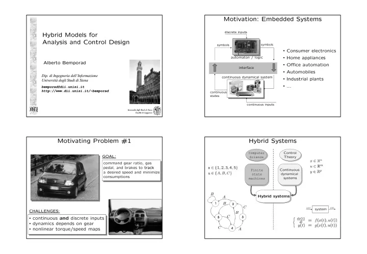
Motivation: Embedded Systems Motivation: Embedded Systems

symbols symbols continuous states continuous inputs

automaton / logic interface

• Consumer electronics
• Home appliances
• Office automation
• Automobiles
• Industrial plants
• ...

Motivating Problem #1 Motivating Problem #1

GOAL GOAL: command gear ratio, gas pedal, and brakes to trac ack k a desired speed and minimize consumptions CHALLE LLENG NGES:

• continuous and discrete inputs
• dynamics depends on gear
• nonlinear torque/speed maps

Hybrid systems

Hybrid Systems Hybrid Systems

Computer Science Control Theory Finite state machines Continuous dynamical systems system

u(t) y(t)

A B C C A B B C

linear systems nonlinear systems linear hybrid systems

?

Key Requirements for Hybrid Models Key Requirements for Hybrid Models

• Des

Descriptive enough to capture the behavior of the system – continuous dynamics (physical laws) – logic components (switches, automata, software code) – interconnection between logic and dynamics

• Si

Simple enough for solving analysis and synthesis problems

Piecewise Affine Systems Piecewise Affine Systems

• Approximates nonlinear dynamics arbitrarily well
• Suitable for stability analysis, reachability analysis

(verification), controller synthesis, ...

(Sontag 1981)

state+input space

Discrete Hybrid Automata Discrete Hybrid Automata

(Torrisi, Bemporad, 2003)

Discrete Hybrid Automata Discrete Hybrid Automata

(Torrisi, Bemporad, 2003)

Switched Affine System

Discrete Hybrid Automata Discrete Hybrid Automata

(Torrisi, Bemporad, 2003)

Event Generator

Discrete Hybrid Automata Discrete Hybrid Automata

(Torrisi, Bemporad, 2003)

Finite State Machine Discrete dynamics evolving according to a Boolean state update function

Discrete Hybrid Automata Discrete Hybrid Automata

(Torrisi, Bemporad, 2003)

Mode Selector a Boolean function selects the active mode i(k) of the SAS

Glover 1975, Williams 1977

Logic and Inequalities Logic and Inequalities

Aî ô B, î ∈ {0, 1} V

j=1 m

W

i∈Pj Xi

W

i∈Nj X

ö i ð ñ

• 1. Convert to Conjunctive Normal Form (CNF):

1 ô X

i∈P1

îi + X

i∈N1

(1 à îi) . . . . . . . . . 1 ô X

i∈Pm

îi + X

i∈Nm

(1 à îi)

• 2. Transform into inequalities:

Every logic proposition can be translated into linear integer inequalities

• 0. Given a Boolean statement F(X1, X2, . . ., Xn)

Logic Logic → → Inequalities: Symbolic Approach Inequalities: Symbolic Approach

Geometric approach: The polytope is the convex hull of the rows of the truth table

Every logic proposition can be translated into linear integer inequalities P,{î : Aî ô B}

T

Aî ô B, î ∈ {0, 1}n

Logic Logic → → Inequalities: Geometric Approach Inequalities: Geometric Approach

Example: logic “AND” Convex hull algorithms: cdd, lrs, qhull, chD, Hull, Porto

3 1 2

conv " # , 1 " # , 1 " # , 1 1 1 " # ! = î : à î1 + î3 ô 0 à î2 + î3 ô 0 î1 + î2 à î3 ô 1      

Key idea: White points cannot be in the hull of black points

Logic Logic → → Inequalities: Geometric Approach Inequalities: Geometric Approach Mixed Logical Dynamical Systems Mixed Logical Dynamical Systems

DHA

• Computationally oriented (Mixed Integer Programming)
• Suitable for optimal controller synthesis, verification, ...

Continuous and binary variables

(Bemporad, Morari 1999)

Mixed Logical Dynamical (MLD) Systems

M = à m = 10 ï > 0 small

• Associate

A Simple Example A Simple Example

• System:
• Then
• Rewrite as a linear equation

and transform x(t + 1) = 0.8x(t) + u(t) if x(t) õ 0 à 0.8x(t) + u(t) if x(t) < 0 ú [î(t) = 1] ↔ [x(t) õ 0] x(t + 1) = 1.6î(t)x(t) à 0.8x(t) + u(t) z(t) = î(t)x(t)

à 10 ô x(t) ô 10, à 1 ô u(t) ô 1 à mî(t) ô x(t) à m à (M + ï)î(t) ô à x(t) à ï z(t) ô Mî(t) z(t) õ mî(t) z(t) ô x(t) à m(1 à î(t)) z(t) õ x(t) à M(1 à î(t)) x(t + 1) = 1.6z(t) à 0.8x(t) + u(t)

HYSDEL HYSDEL

( (HYbrid HYbrid Systems Systems DEscription DEscription Language) Language)

• Describe hybrid systems:

– Automata – Logic – Lin. Dynamics – Interfaces – Constraints

(Torrisi, Bemporad, 2003)

• Automatically generate MLD models in Matlab

http://www.dii.unisi.it/~bemporad/tools.html http://control.ethz.ch/~hybrid/hysdel

Download:

Example 1: AD section Example 1: AD section

[ ] [ ]

max

s h h = ↔ ≥ T

SYSTEM tank { INTERFACE { STATE { REAL h [-0.3,0.3]; } INPUT { REAL Q [-10,10]; } PARAMETER { REAL k = 1; REAL e = 1e-6; } } /* end interface */ IMPLEMENTATION { AUX { BOOL s; } AD { s = hmax - h <= 0; } CONTINUOUS { h = h + k * Q; } } /* end implementation */ } /* end system */

Example 2: DA section Example 2: DA section

( ) 2.3 1.3 ( )

t comp t t

u u u u u u u u <  =  − ≥ 

SYSTEM motor { INTERFACE { STATE { REAL ucomp; } INPUT { REAL u [0,10]; } PARAMETER { REAL ut = 1; REAL e = 1e-6;} } /* end interface */ IMPLEMENTATION { AUX { REAL unl; BOOL th; } AD { th = ut - u <= 0; } DA { unl = { IF th THEN 2.3*u - 1.3*ut ELSE u }; } CONTINUOUS { ucomp = unl; } } /* end implementation */ } /* end system */

Nonlinear amplification unit

Example 3: LOGIC section Example 3: LOGIC section

( )

brake alarm tunnel fire

u u s s = ∧ ¬ ∨ ¬

fire alarm

s u →

SYSTEM train { INTERFACE { STATE { BOOL brake; } INPUT { BOOL alarm, tunnel, fire; } } /* end interface */ IMPLEMENTATION { AUX { BOOL decision; } LOGIC { decision = alarm & (~tunnel | ~fire); } AUTOMATA { brake = decision; } MUST { fire -> alarm; } } /* end implementation */ } /* end system */

Example 4: CONTINUOUS section Example 4: CONTINUOUS section

( ) d i C u t dt =

( 1) ( ) ( ) T u k u k i k C + = +

Apply forward difference rule:

SYSTEM capacitorD { INTERFACE { STATE { REAL u; } PARAMETER { REAL R = 1e4; REAL C = 1e-4; REAL T = 1e-1; } } /* end interface */ IMPLEMENTATION { CONTINUOUS { u = u - T/C/R*i; } } /* end implementation */ } /* end system */

Example 5: AUTOMATA section Example 5: AUTOMATA section

SYSTEM outflow { INTERFACE { STATE { BOOL closing, stop, opening; } INPUT { BOOL uclose, uopen, ustop; } } /* end of interface */ IMPLEMENTATION { AUTOMATA { closing = (uclose & closing) | (uclose & stop); stop = ustop | (uopen & closing) | (uclose & opening);

• pening = (uopen & stop) | (uopen & opening); }

MUST { ~(uclose & uopen); ~(uclose & ustop); ~(uopen & ustop); } } /* end implementation */ } /* end system */

Example 6: MUST section Example 6: MUST section

max

h h ≤ ≤

SYSTEM watertank { INTERFACE { STATE { REAL h; } INPUT { REAL Q; } PARAMETER { REAL hmax = 0.3; REAL k = 1; } } /* end interface */ IMPLEMENTATION { CONTINUOUS { h = h + k*Q; } MUST { h - hmax <= 0;

• h <= 0; }

} /* end implementation */ } /* end system */

Modeling Flow Modeling Flow

x(t + 1) = A1x(t) + B1u(t) + f1 A2x(t) + B2u(t) + f2 x(t + 1) = A3x(t) + B3u(t) + f3 x(t + 1) = g12x(t) + h12u(t) < k12 g32x(t) + h32u(t) < k32 g23x(t) + h23u(t) < k23 g13x(t) + h13u(t) < k13

A/D D/A continuous logic

Designer Hysdel

MLD PWA HYSDEL Source

Piecewise Affine form Mixed Logical Dynamical form

Example: Bouncing Ball Example: Bouncing Ball

F= m g

x ¨ = à g x ô 0 ⇒ x ç(t+) = à (1 à ë)x ç (tà)

How to model this system in MLD form? ë ∈ [0, 1]

x N

HYSDEL HYSDEL -

• Bouncing Ball

Bouncing Ball

SYSTEM bouncing_ball { INTERFACE {

/* Description of variables and constants */

STATE { REAL height [-10,10]; REAL velocity [-100,100]; } PARAMETER { REAL g=9.8; REAL dissipation=.4; /* 0=elastic, 1=completely anelastic */ REAL Ts=.05; } } IMPLEMENTATION { AUX { REAL z1; REAL z2; BOOL negative; } AD { negative = height <= 0; } DA { z1 = { IF negative THEN height-Ts*velocity ELSE height+Ts*velocity-Ts*Ts*g}; z2 = { IF negative THEN -(1-dissipation)*velocity ELSE velocity-Ts*g}; } CONTINUOUS { height = z1; velocity=z2;} }}

System Theory for Hybrid Systems System Theory for Hybrid Systems

• Analysis

– Well-posedness – Realization & Transformation – Reachability (=Verification) – Observability – Stability

• Synthesis

– Control – State estimation – Identification – Modeling language

Well Well-

• posedness

posedness

• MLD well-posedness :

are single valued î(t) = F(x(t), u(t)) z(t) = G(x(t), u(t)) {x(t), u(t)} → {x(t + 1)} {x(t), u(t)} → {y(t)}

Numerical test based on mixed-integer programming available

(Bemporad, Morari, Automatica, 1999)

Are state and output trajectories defined ? Uniquely defined ? Persistently defined ?

Realization and Transformation Realization and Transformation (State (State-

• Space Hybrid Models)

Space Hybrid Models) Other Existing Hybrid Models Other Existing Hybrid Models

• Linear complementarity (LC) systems

x(t + 1) = Ax(t) + B1u(t) + B2w(t) y(t) = Cx(t) + D1u(t) + D2w(t) v(t) = E1x(t) + E2u(t) + E3w(t) + e4 0 ô v(t)⊥w(t) õ 0

Ex: mechanical systems circuits with diodes etc.

• Extended linear complementarity (ELC) systems
• Min-max-plus-scaling (MMPS) systems

M := xi|ë| max(M1, M2)| min(M1, M2)|M1 + M2|ìM1

x(t + 1) = Mx(x(t), u(t), d(t)) y(t) = My(x(t), u(t), d(t)) 0 õ Mc(x(t), u(t), d(t))

MMPS function: defined by the grammar

Generalization of LC systems

x(t + 1) = 2 max(x(t), 0) + min(à 2

1u(t), 1)

Example:

Used for modeling discrete-event systems (t=event counter)

(De Schutter, Van den Boom, 2000) (De Schutter, De Moor, 2000) (Heemels, 1999)

Equivalences of Hybrid Models Equivalences of Hybrid Models

Σ1 Σ2

x(0)=x(0) u(k) x(k), y(k) x(k), y(k)

Equivalence Results Equivalence Results

(Heemels, De Schutter, Bemporad, Automatica, 2001)

Theoretical properties and analysis/synthesis tools can be transferred from one class to another

MLD PWA MMPS ELC LC ? ? ? ? ? ? ? ? DHA ? (Torrisi, Bemporad, IEEE CST, 2003) (Bemporad and Morari, Automatica, 1999) (Bemporad, Ferrari-T.,Morari, IEEETAC, 2000)

MLD and LC Systems MLD and LC Systems

(Heemels, De Schutter, Bemporad, Automatica, 2001)

Set and substitute For each complementarity pair introduce a binary variable

vi(t), wi(t) îi(t) ∈ {0, 1} [îi(t) = 1] → [vi(t) = 0, wi(t) õ 0] [îi(t) = 0] → [vi(t) õ 0, wi(t) = 0] wi(t) ô Mîi(t) vi(t) ô M(1 à îi(t)) wi(t) õ 0 vi(t) õ 0

x(t + 1) = Ax(t) + B1u(t) + B2w(t) y(t) = Cx(t) + D1u(t) + D2w(t) v(t) = E1x(t) + E2u(t) + E3w(t) + e4 0 ô v(t)⊥w(t) õ 0 x(t + 1) = Ax(t) + B1u(t) y(t) = Cx(t) + D1u(t) + B2î(t) + B3z(t) + D2î(t) + D3z(t) E2î(t) + E3z(t) ô E4x(t) + E1u(t) + E5

zi(t) = wi(t) v(t) = E1x(t) + E2u(t) + E3w(t) + e4 Proof:

MLD and PWA Systems MLD and PWA Systems

• MLD:

PWA form

• By well-posedness hypothesis on + linearity of

MLD constraints

x(t + 1) = Ax(t) + B1u(t) + B2î(t) + B3z(t) y(t) = Cx(t) + D1u(t) + D2î(t) + D3z(t) E2î(t) + E3z(t) ô E1u(t) + E4x(t) + E5

z(t), î(t) z = Ki

4x + Ki 1u + Ki 5

∀(x, u) : F(x, u) = îi

x(t + 1) = Aix(t) + Biu(t) + fi y(t) = Cix(t) + Diu(t) + gi Fix(t) + Giu(t) ô hi

• Confirms (Sontag, 1996): PWL systems and hybrid systems

are equivalent

(Bemporad, Ferrari-Trecate, Morari, IEEE TAC,2000)

Theorem MLD systems and PWA systems are equivalent

Efficient MLD to PWA Conversion Efficient MLD to PWA Conversion

• Proof is constructive: given an MLD system it returns its

equivalent PWA form

• Drawback: it needs the enumeration of all possible

combinations of binary states, binary inputs, and δ variables

• Most of such combinations lead to empty regions
• Efficient algorithms are available for converting MLD models

into PWA models avoiding such an enumeration:

• A. Bemporad, “A Recursive Algorithm for Converting Mixed Logical

Dynamical Systems into an Equivalent Piecewise Affine Form”, IEEE

• Trans. Autom. Contr., October 2003.
• T. Geyer, F.D. Torrisi and M. Morari, “Efficient Mode Enume-

ration of Compositional Hybrid Models”, HSCC’03

MLD to PWA Conversion Algorithm MLD to PWA Conversion Algorithm

No Note: the cells Ωi are embedded in Rn+m by treating integer states and integer inputs as continuous vars: xb,ub ∈ [0,1] → xb,ub ∈ [-1/2,1/2) ∪ [1/2,3/2]

GO GOAL: split a given set B of states+inputs into polyhedral cells and find the affine dynamics in each cell, therefore determining the PWA system which is equivalent to the given MLD system

B

x u

(Bemporad, 2002)

MLD MLD to to PWA PWA Conversion Conversion -

• Start

Start

• Let (x*,u*) be a given point in B

(e.g.: (x*,u*) is the Chebychev center

• f B, computable via LP)

B

x u (x*,u*)

• Problem: (x*,u*) may not be 0/1 valued
• Find (x1,u1) which is closest to (x*,u*), is integer feasible,

and satisfies the MLD constraints:

Mi Mixed xed In Integer Li Linear ar Progr

• gram

am (M (MIL ILP)

MLD MLD to to PWA PWA Conversion Conversion

Now fix δ=δ1. To find the polyhedral cell Ωi and dynamics (Ai,Bi,fi):

• 1. From MLD constraints, compute

B

x u (x*,u*)

• 2. Substitute z(k) in the MLD dynamics
• 3. Find polyhedral cell Ωi

MLD MLD to to PWA PWA Conversion Conversion -

• Partition

Partition

The Theore rem: is a partition of B

Ωi

(x*,u*)

• R1

R2 RN R3 B R4

Proceed iteratively: for each region Ri repeat the whole procedure with B∩Ri

Note: similar to multiparametric Quadratic Programming algorithm

(Bemporad et al., 2002)

x u

Now partition the rest of the space B\Ωi

MLD MLD to to PWA PWA Conversion Conversion -

• Union

Union

Regions where the affine dynamics is the same can be joined (when their union is convex).

(Bemporad, Fukuda, Torrisi, 2001)

• 2.5
• 2
• 1.5
• 1
• 0.5

0.5 1 1.5 2 2.5

• 2.5
• 2
• 1.5
• 1
• 0.5

0.5 1 1.5 2 2.5 CR1 CR2 CR3 CR4 CR5 CR6 CR7 CR8 CR9

• 2.5
• 2
• 1.5
• 1
• 0.5

0.5 1 1.5 2 2.5

• 2.5
• 2
• 1.5
• 1
• 0.5

0.5 1 1.5 2 2.5 CR1 CR2 CR3 CR4 CR5 CR6 CR7

Example: Heat and Cool Example: Heat and Cool

Cold air flow Hot air flow

#1 #2 T1 T2 Tamb

Rules o s of the the ga game: me:

Hybrid HYSDEL Model Hybrid HYSDEL Model Hybrid MLD Model Hybrid MLD Model

• MLD model
• 2 continuous states:
• 1 continuous input:
• 6 auxiliary binary vars:
• 2 auxiliary continuous vars:

(room temperature Tamb) (temperatures T1,T2) (water flows uhot, ucold) (4 thresholds + 2 for OR condition)

• 20 mixed-integer inequalities

Possible combination of integer variables: 26 = 64

Hybrid PWA Model Hybrid PWA Model

• PWA model
• 2 continuous states:
• 1 continuous input:

(room temperature Tamb) (temperatures T1,T2)

• 5 polyhedral regions

(partition does not depend on input)

Computation time: 0.72 s in Matlab

uhot = ¯ UH ucold = uhot = ucold = ¯ UC uhot = ucold =

• 10

10 20 30 40 50

• 10

10 20 30 40 50 Temperature T

1 (deg C)

Temperature T

2 (deg C)

Why are we interested in getting MLD Why are we interested in getting MLD and PWA models ? and PWA models ? Major Advantage of MLD Framework Major Advantage of MLD Framework

Many problems of analysis: – Stability – Safety – Controllability – Observability Many problems of synthesis: – Controller design – Filter design / Fault detection & state estimation can be expressed as (mixed integer) mathematical programming problems for which many algorithms and software tools exist. (However, all these problems are NP-hard !)

Hybrid Models Hybrid Models

Task Model Modeling DHA Simulation DHA Control MLD,PWA,MMPS Stability PWA Verification PWA Identification PWA Fault Detection MLD Estimation MLD Each model is most advantageous depending on task: