Mothers Major Depression when Children were at Age 2, 3, 5, and 9 - - PDF document

SLIDE 1

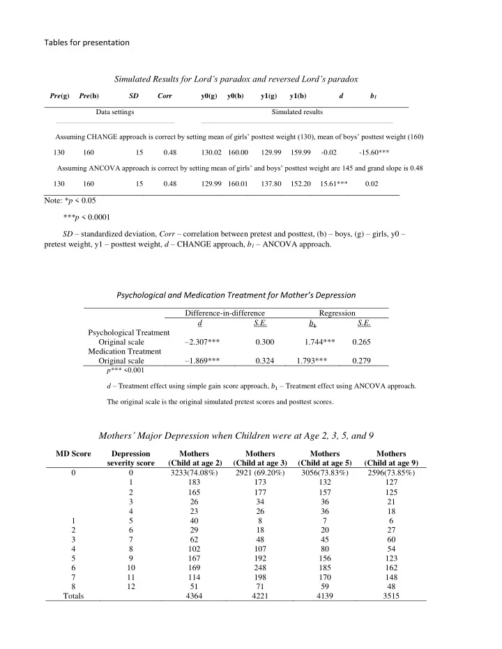
Tables for presentation Simulated Results for Lord’s paradox and reversed Lord’s paradox

Pre(g) Pre(b) SD Corr y0(g) y0(b) y1(g) y1(b) d b1 Data settings Simulated results Assuming CHANGE approach is correct by setting mean of girls’ posttest weight (130), mean of boys’ posttest weight (160) 130 160 15 0.48 130.02 160.00 129.99 159.99

• 0.02
• 15.60***

Assuming ANCOVA approach is correct by setting mean of girls’ and boys’ posttest weight are 145 and grand slope is 0.48 130 160 15 0.48 129.99 160.01 137.80 152.20 15.61*** 0.02

Note: *p < 0.05 ***p < 0.0001 SD – standardized deviation, Corr – correlation between pretest and posttest, (b) – boys, (g) – girls, y0 – pretest weight, y1 – posttest weight, d – CHANGE approach, b1 – ANCOVA approach.

Psychological and Medication Treatment for Mother’s Depression

Difference-in-difference Regression d S.E. 𝑐1 S.E. Psychological Treatment Original scale –2.307*** 0.300 1.744*** 0.265 Medication Treatment Original scale –1.869*** 0.324 1.793*** 0.279

p*** <0.001 d – Treatment effect using simple gain score approach, 𝑐1 – Treatment effect using ANCOVA approach. The original scale is the original simulated pretest scores and posttest scores.

Mothers’ Major Depression when Children were at Age 2, 3, 5, and 9

MD Score Depression severity score Mothers (Child at age 2) Mothers (Child at age 3) Mothers (Child at age 5) Mothers (Child at age 9) 3233(74.08%) 2921 (69.20%) 3056(73.83%) 2596(73.85%) 1 183 173 132 127 2 165 177 157 125 3 26 34 36 21 4 23 26 36 18 1 5 40 8 7 6 2 6 29 18 20 27 3 7 62 48 45 60 4 8 102 107 80 54 5 9 167 192 156 123 6 10 169 248 185 162 7 11 114 198 170 148 8 12 51 71 59 48 Totals 4364 4221 4139 3515

SLIDE 2

Simulation Results for Lord’s Paradox and Reversed Paradox, Varying Normality, SD, Slope Correlation, & Independence of Pretest Weight from Gender

Normality SD(g) SD(b) Corr(g) Corr(b) y0(g) y0(b) y1(g) y1(b) d 𝒄𝟐 Data settings Simulated results Pretest means are different: mean of girls’ pretest weight (130), mean of boys’ pretest weight (160) Assuming the simple gain score null H0 is correct, with mean of girls’ posttest weight to 130, & mean of boys’ posttest weight to 160 Yes 15 15 0.48 0.48 130.02 160.00 129.99 159.99

• 0.02
• 15.60***

Yes 5 15 0.48 0.48 130.01 160.00 130.00 159.99 0.00

• 15.60***

Yes 15 15 0.48 130.02 160.00 129.98 159.99

• 0.03
• 22.81***

Yes 15 15 0.48 130.02 160.01 129.99 159.99

• 0.01
• 22.79***

Yes 5 15 0.48 130.01 160.00 129.99 159.99 0.00

• 17.05***

Yes 5 15 0.48 130.01 160.01 130.00 159.99 0.01

• 28.54***

No 15 15 0.48 0.48 85.00 92.50 82.00 88.00 1.50

• 5.96***

No 5 15 0.48 0.48 85.00 92.50 82.00 88.00 1.50

• 5.97***

No 15 15 0.48 85.00 92.50 82.00 88.00 1.51

• 5.97***

No 15 15 0.48 85.00 92.50 82.01 88.00 1.50

• 5.97***

No 5 15 0.48 85.00 92.50 82.00 88.00 1.50

• 5.98***

No 5 15 0.48 85.00 92.50 82.00 88.00 1.51

• 5.99***

Assuming the ANCOVA null H0 is correct by setting means of girls’ and boys’ posttest weights to those predicted by slope of 0.48 Yes 15 15 0.48 0.48 129.99 160.01 137.80 152.20 15.61*** 0.02 Yes 5 15 0.48 0.48 130.00 160.01 137.80 152.20 15.61*** 0.05 No 5 15 0.48 0.48 85.00 92.50 83.56 86.44 4.63

• 2.86

No 15 15 0.48 0.48 84.99 92.50 83.56 86.44 4.63

• 2.84

Pretest means are the same: mean of girls’ pretest weight (145), mean of boys’ pretest weight (145) Assuming the simple gain score null H0 is correct by setting the means of girls’ and boys’ posttest weights to 145 Yes 5 15 0.48 0.48 145.00 145.01 145.00 145.00 0.01 0.00 Yes 15 15 0.48 0.48 144.99 145.01 145.00 145.00 0.01 0.00 No 5 15 0.48 0.48 88.75 88.75 85.00 85.00 0.01 0.00 No 15 15 0.48 0.48 88.74 88.75 85.00 85.00 0.01 0.00 Assuming alternative HA is correct, setting the mean of girls’ posttest weight to 130 & the mean of boys’ posttest weight to 160 Yes 5 15 0.48 145.01 145.00 129.99 159.99 -30.00***

• 30.00***

Yes 15 15 0.48 145.02 145.00 129.98 159.99 -30.03***

• 30.02***

Yes 5 15 0.48 145.01 145.01 130.00 159.99 -29.99***

• 30.00***

Yes 15 15 0.48 145.02 145.01 129.99 159.99 -30.01***

• 30.01***

Yes 5 15 0.48 0.48 145.01 145.00 130.00 159.99 -30.00***

• 30.00***

Yes 15 15 0.48 0.48 145.02 145.00 129.99 159.99 -30.02***

• 30.01***

No 5 15 0.48 88.75 88.75 82.00 88.00

• 6.00*
• 5.99***

No 15 15 0.48 88.75 88.75 82.01 88.00

• 6.00*
• 5.99***

No 5 15 0.48 88.75 88.75 82.00 88.00

• 5.99*
• 5.99***

No 15 15 0.48 88.75 88.75 82.00 88.00

• 5.99*
• 5.99***

No 5 15 0.48 0.48 88.75 88.75 82.00 88.00

• 6.00*
• 5.99***

No 15 15 0.48 0.48 88.75 88.75 82.00 88.00

• 6.00*
• 5.99***

Note: *p < .05. ***p < .0001 Normality – normal distribution, SD – standard deviation, Corr – correlation between pretest and posttest, (b) – boys, (g) – girls, y0 – pretest weight, y1 – posttest weight, d – CHANGE approach, 𝑐1 – ANCOVA approach. The first bold font is Lord’s paradox and the second bold font is Lord’s paradox reversed.

SLIDE 3

Table 3

Simulation Results on Varying Pretest and Posttest Different for Girls

y0(g) y1(g) y0(g) y0(b) y1(g) y1(b) d

b1

Data setting Simulated data Analysis results 130 130 130.02 160.00 129.99 159.99

• 0.02
• 15.60***

135 130 135.02 160.00 129.99 159.99

• 5.02***
• 18.00***

140 130 140.02 160.00 129.99 159.99

• 10.02***
• 20.40***

145 130 145.02 160.00 129.99 159.99

• 15.02***
• 22.81***

150 130 150.02 160.00 129.99 159.99

• 20.02***
• 25.21***

155 130 155.02 160.00 129.99 159.99

• 25.02***
• 27.61***

160 130 160.02 160.00 129.99 159.99

• 30.02***
• 30.01***

130 135 130.02 160.00 134.99 159.99 4.98***

• 10.60***

135 135 135.02 160.00 134.99 159.99

• 0.02
• 13.00***

140 135 140.02 160.00 134.99 159.99

• 5.02***
• 15.40***

145 135 145.02 160.00 134.99 159.99

• 10.02***
• 17.81***

150 135 150.02 160.00 134.99 159.99

• 15.02***
• 20.21***

155 135 155.02 160.00 134.99 159.99

• 20.02***
• 22.61***

160 135 160.02 160.00 134.99 159.99

• 25.02***
• 25.01***

130 140 130.02 160.00 139.99 159.99 9.98***

• 5.60***

135 140 135.02 160.00 139.99 159.99 4.98***

• 8.00***

140 140 140.02 160.00 139.99 159.99

• 0.02
• 10.40***

145 140 145.02 160.00 139.99 159.99

• 5.02***
• 12.81***

150 140 150.02 160.00 139.99 159.99

• 10.02***
• 15.21***

155 140 155.02 160.00 139.99 159.99

• 15.02***
• 17.61***

160 140 160.02 160.00 139.99 159.99

• 20.02***
• 20.01***

130 145 130.02 160.00 144.99 159.99 14.98***

• 0.60

135 145 135.02 160.00 144.99 159.99 9.98***

• 3.00*

140 145 140.02 160.00 144.99 159.99 4.98***

• 5.40***

145 145 145.02 160.00 144.99 159.99

• 0.02
• 7.81***

150 145 150.02 160.00 144.99 159.99

• 5.02***
• 10.21***

155 145 155.02 160.00 144.99 159.99

• 10.02***
• 12.61***

160 145 160.02 160.00 144.99 159.99

• 15.02***
• 15.01***

130 150 130.02 160.00 149.99 159.99 19.98*** 4.40** 135 150 135.02 160.00 149.99 159.99 14.98*** 2.00

SLIDE 4

140 150 140.02 160.00 149.99 159.99 9.98***

• 0.40

145 150 145.02 160.00 149.99 159.99 4.98***

• 2.81*

150 150 150.02 160.00 149.99 159.99

• 0.02
• 5.21***

155 150 155.02 160.00 149.99 159.99

• 5.02***
• 7.61***

160 150 160.02 160.00 149.99 159.99

• 10.02***
• 10.01***

130 155 130.02 160.00 154.99 159.99 24.98*** 9.40*** 135 155 135.02 160.00 154.99 159.99 19.98*** 7.00*** 140 155 140.02 160.00 154.99 159.99 14.98*** 4.60*** 145 155 145.02 160.00 154.99 159.99 9.98*** 2.19a 150 155 150.02 160.00 154.99 159.99 4.98***

• 0.21

155 155 155.02 160.00 154.99 159.99

• 0.02
• 2.61*

160 155 160.02 160.00 154.99 159.99

• 5.02***
• 5.01***

130 160 130.02 160.00 159.99 159.99 29.98*** 14.40*** 135 160 135.02 160.00 159.99 159.99 24.98*** 12.00*** 140 160 140.02 160.00 159.99 159.99 19.98*** 9.60*** 145 160 145.02 160.00 159.99 159.99 14.98*** 7.19*** 150 160 150.02 160.00 159.99 159.99 9.98*** 4.79*** 155 160 155.02 160.00 159.99 159.99 4.98*** 2.39* 160 160 160.02 160.00 159.99 159.99

• 0.02
• 0.01

Note: ap < .1, *p < .05, **p < .001, ***p < .0001 (b) –boys, (g) –girls, y0 –pretest weight, y1–posttest weight, d – CHANGE approach, 𝑐1 – ANCOVA approach. Data setting: boys pretest/posttest mean = 160, slope for boys/girls = 0.48, standard deviation = 15. The italic font are results in opposite directions. The first bold font is Lord’s paradox and the second bold font is Lord’s paradox reversed.

SLIDE 5

Cross-Lagged Panel Model of Mothers’ Depression Featuring Wave 3, 4, and 5 Latent Growth Model of Mothers’ Depression Featuring Wave 3, 4, and 5 Depression4 Depression5 PSY_TRT3 PSY_TRT4 MED_TRT3 MED_TRT4 Depression3 Depression3 Depression4 Depression5 Depression3 Depression4 Depression5 Intercept Slope 1 PSY_TRT3 PSY_TRT4 Slope 2 MED_TRT4 MED_TRT3 Intercept Slope 1 Slope 2 Depression3 Depression4 Depression5

SLIDE 6

Cross-Lagged Panel Model of Mothers’ Depression Featuring Wave 3, 4, and 5 Latent Growth Model of Mothers’ Depression Featuring Wave 3, 4, and 5

0.233*** 0.221*** 0.104*** 0.371*** 0.112*** 0.218*** 0.368*** 0.118*** 0.220*** 0.042* 0.083*** 0.066*** 0.321***

PSY_TRT3

• 0.156***

0.269*** 0.087*** 0.212***

• 0.036*

Depression3 Depression4 Depression5 Intercept Slope 1 PSY_TRT4 Slope 2

0.355*** 0.252***

Depression4 Depression5 PSY_TRT3 PSY_TRT4 MED_TRT3 MED_TRT4 Depression3 Depression3 Depression4 Depression5

0.244***

MED_TRT4 Intercept

0.123***

• 0.102***

0.403*** 0.069***

• 0.056***

MED_TRT3 Slope 1 Slope 2 Depression3 Depression4 Depression5

SLIDE 7

Cross-lagged panel model: psychological treatment

Title: Cross-legged panel model; Data: file is Trt_Depr_y2y3y5y9.csv; variable: names are idnum TxDepW3 MedDepW3 TxDepW4 MedDepW4 TxDepW5 MedDepW5 depress_md2 depress2 depress_md3 depress3 depress_md4 depress4 depress_md5 depress5; Missing are all (-9999); usevariables are TxDepW3 TxDepW4 depress3 depress4 depress5; model: TxDepW4 ON TxDepW3 depress3; depress4 ON TxDepW3 depress3; !TxDepW5 ON TxDepW4 depress4; depress5 ON TxDepW4 depress4 depress3; depress3 WITH TxDepW3; depress4 WITH TxDepW4; !depress5 WITH TxDepW5;

• utput: stdyx samp mod residual;

STDYX Standardization Two-Tailed Estimate S.E. Est./S.E. P-Value TXDEPW4 ON TXDEPW3 0.252 0.017 15.139 0.000 DEPRESS3 0.112 0.016 6.918 0.000 DEPRESS4 ON TXDEPW3 0.042 0.017 2.466 0.014 DEPRESS3 0.371 0.015 25.008 0.000 DEPRESS5 ON TXDEPW4 0.104 0.017 6.147 0.000 DEPRESS4 0.220 0.018 12.215 0.000 DEPRESS3 0.221 0.017 13.037 0.000 DEPRESS3 WITH TXDEPW3 0.323 0.015 21.739 0.000 DEPRESS4 WITH TXDEPW4 0.333 0.014 23.739 0.000 Means TXDEPW3 0.235 0.017 14.213 0.000 DEPRESS3 0.561 0.016 34.077 0.000 Intercepts TXDEPW4 0.131 0.018 7.510 0.000 DEPRESS4 0.284 0.018 16.062 0.000 DEPRESS5 0.234 0.019 12.033 0.000 Variances TXDEPW3 1.000 0.000 999.000 999.000 DEPRESS3 1.000 0.000 999.000 999.000 Residual Variances TXDEPW4 0.906 0.009 98.029 0.000 DEPRESS4 0.851 0.011 80.693 0.000 DEPRESS5 0.829 0.012 71.303 0.000 R-SQUARE Observed Two-Tailed Variable Estimate S.E. Est./S.E. P-Value TXDEPW4 0.094 0.009 10.210 0.000 DEPRESS4 0.149 0.011 14.147 0.000 DEPRESS5 0.171 0.012 14.733 0.000

SLIDE 8

Cross-lagged panel model: medication treatment Title: Cross-legged panel model;

Data: file is Trt_Depr_y2y3y5y9.csv; variable: names are idnum TxDepW3 MedDepW3 TxDepW4 MedDepW4 TxDepW5 MedDepW5 depress_md2 depress2 depress_md3 depress3 depress_md4 depress4 depress_md5 depress5; Missing are all (-9999); usevariables are MedDepW3 MedDepW4 depress3 depress4 depress5; model: MedDepW4 ON MedDepW3 depress3; depress4 ON MedDepW3 depress3; !MedDepW5 ON MedDepW4 depress4; depress5 ON MedDepW4 depress4 depress3; depress3 WITH MedDepW3; depress4 WITH MedDepW4; !depress5 WITH MedDepW5;

• utput: std samp mod residual;

STDYX Standardization Two-Tailed Estimate S.E. Est./S.E. P-Value MEDDEPW4 ON MEDDEPW3 0.355 0.015 23.513 0.000 DEPRESS3 0.118 0.015 7.717 0.000 DEPRESS4 ON MEDDEPW3 0.066 0.016 4.011 0.000 DEPRESS3 0.368 0.014 25.538 0.000 DEPRESS5 ON MEDDEPW4 0.083 0.016 5.109 0.000 DEPRESS4 0.233 0.018 13.280 0.000 DEPRESS3 0.218 0.017 12.740 0.000 DEPRESS3 WITH MEDDEPW3 0.260 0.015 16.847 0.000 DEPRESS4 WITH MEDDEPW4 0.259 0.015 17.482 0.000 Means MEDDEPW3 0.210 0.016 12.724 0.000 DEPRESS3 0.561 0.016 34.077 0.000 Intercepts MEDDEPW4 0.089 0.017 5.238 0.000 DEPRESS4 0.282 0.018 15.955 0.000 DEPRESS5 0.237 0.020 12.125 0.000 Variances MEDDEPW3 1.000 0.000 999.000 999.000 DEPRESS3 1.000 0.000 999.000 999.000 Residual Variances MEDDEPW4 0.838 0.011 74.329 0.000 DEPRESS4 0.848 0.011 79.770 0.000 DEPRESS5 0.832 0.012 72.193 0.000 R-SQUARE Observed Two-Tailed Variable Estimate S.E. Est./S.E. P-Value MEDDEPW4 0.162 0.011 14.339 0.000 DEPRESS4 0.152 0.011 14.318 0.000 DEPRESS5 0.168 0.012 14.542 0.000

SLIDE 9

Latent growth model: psychological treatment

Title: Cross-legged panel model; Data: file is Trt_Depr_y2y3y5y9.csv; variable: names are idnum TxDepW3 MedDepW3 TxDepW4 MedDepW4 TxDepW5 MedDepW5 depress_md2 depress2 depress_md3 depress3 depress_md4 depress4 depress_md5 depress5; Missing are all (-9999); usevariables are TxDepW3 TxDepW4 depress3 depress4 depress5; analysis: estimator=ml; model: !I S | depress3@0 depress4* depress5@1; I BY depress3@1 depress4@1 depress5@1; S1 BY depress3@-1 depress4@0; S2 BY depress4@0 depress5@1; I ON TxDepW3 TxDepW4; S1 ON TxDepW3; S2 ON TxDepW4; TxDepW4 ON TxDepW3 S1; I WITH S1 S2; S1 WITH S2; [I* S1* S2*]; depress3@0; depress4@0; depress5@0; [depress3@0]; [depress4@0]; [depress5@0]; Plot: Type=Plot3;

• utput: stdyx samp mod residual;

STDYX Standardization Two-Tailed Estimate S.E. Est./S.E. P-Value I BY DEPRESS3 0.925 0.015 63.709 0.000 DEPRESS4 1.000 0.000 999.000 999.000 DEPRESS5 0.996 0.017 59.272 0.000 S1 BY DEPRESS3 -1.079 0.015 -73.943 0.000 DEPRESS4 0.000 0.000 999.000 999.000 S2 BY DEPRESS4 0.000 0.000 999.000 999.000 DEPRESS5 1.147 0.017 65.775 0.000 I ON TXDEPW3 0.087 0.013 6.472 0.000 TXDEPW4 0.269 0.014 19.132 0.000 S1 ON TXDEPW3 -0.156 0.015 -10.423 0.000 S2 ON TXDEPW4 -0.036 0.017 -2.109 0.035 TXDEPW4 ON S1 0.212 0.016 13.215 0.000 TXDEPW4 ON TXDEPW3 0.321 0.015 20.861 0.000 I WITH S1 0.528 0.012 42.342 0.000 S2 -0.580 0.012 -46.949 0.000 S1 WITH S2 -0.445 0.015 -29.574 0.000 Intercepts TXDEPW4 0.199 0.017 11.734 0.000 DEPRESS3 0.000 0.000 999.000 999.000 DEPRESS4 0.000 0.000 999.000 999.000 DEPRESS5 0.000 0.000 999.000 999.000 I 0.403 0.018 22.914 0.000 S1 -0.053 0.017 -3.080 0.002 S2 0.006 0.019 0.335 0.738 Residual Variances

SLIDE 10

TXDEPW4 0.873 0.011 81.658 0.000 DEPRESS3 0.000 999.000 999.000 999.000 DEPRESS4 0.000 999.000 999.000 999.000 DEPRESS5 0.000 999.000 999.000 999.000 I 0.852 0.011 77.543 0.000 S1 0.976 0.005 209.020 0.000 S2 0.992 0.004 229.035 0.000 R-SQUARE Observed Two-Tailed Variable Estimate S.E. Est./S.E. P-Value TXDEPW4 0.127 0.011 11.876 0.000 DEPRESS3 1.000 999.000 999.000 999.000 DEPRESS4 1.000 999.000 999.000 999.000 DEPRESS5 1.000 999.000 999.000 999.000 Latent Two-Tailed Variable Estimate S.E. Est./S.E. P-Value I 0.148 0.011 13.494 0.000 S1 0.024 0.005 5.212 0.000 S2 0.008 0.004 1.826 0.068

Latent growth model: medication treatment

Title: Cross-legged panel model; Data: file is Trt_Depr_y2y3y5y9.csv; variable: names are idnum TxDepW3 MedDepW3 TxDepW4 MedDepW4 TxDepW5 MedDepW5 depress_md2 depress2 depress_md3 depress3 depress_md4 depress4 depress_md5 depress5; Missing are all (-9999); usevariables are MedDepW3 MedDepW4 depress3 depress4 depress5; analysis: estimator=ml; model: !I S | depress3@0 depress4* depress5@1; I BY depress3@1 depress4@1 depress5@1; S1 BY depress3@-1 depress4@0; STDYX Standardization Two-Tailed Estimate S.E. Est./S.E. P-Value I BY DEPRESS3 0.924 0.015 63.664 0.000 DEPRESS4 1.000 0.000 999.000 999.000 DEPRESS5 0.994 0.017 59.116 0.000 S1 BY DEPRESS3 -1.078 0.015 -73.790 0.000 DEPRESS4 0.000 0.000 999.000 999.000 S2 BY DEPRESS4 0.000 0.000 999.000 999.000 DEPRESS5 1.145 0.017 65.658 0.000 I ON MEDDEPW3 0.069 0.014 4.729 0.000 MEDDEPW4 0.244 0.015 16.566 0.000 S1 ON MEDDEPW3 -0.102 0.015 -6.658 0.000

SLIDE 11

S2 BY depress4@0 depress5@1; I ON MedDepW3 MedDepW4; S1 ON MedDepW3; S2 ON MedDepW4; MedDepW4 ON MedDepW3 S1; !S1 WITH MedDepW4; s1 with s2; I WITH S1 S2; S1 WITH S2; [I* S1* S2*]; depress3@0; depress4@0; depress5@0; [depress3@0]; [depress4@0]; [depress5@0]; Plot: Type=Plot3;

• utput: stdyx samp mod residual;

S2 ON MEDDEPW4 -0.056 0.017 -3.362 0.001 MEDDEPW4 ON S1 0.123 0.016 7.825 0.000 MEDDEPW4 ON MEDDEPW3 0.403 0.014 27.861 0.000 I WITH S1 0.528 0.012 42.866 0.000 S2 -0.573 0.012 -46.021 0.000 S1 WITH S2 -0.443 0.015 -29.717 0.000 Intercepts MEDDEPW4 0.159 0.016 9.641 0.000 DEPRESS3 0.000 0.000 999.000 999.000 DEPRESS4 0.000 0.000 999.000 999.000 DEPRESS5 0.000 0.000 999.000 999.000 I 0.420 0.018 23.545 0.000 S1 -0.069 0.017 -4.010 0.000 S2 0.012 0.019 0.620 0.535 Residual Variances MEDDEPW4 0.833 0.012 71.243 0.000 DEPRESS3 0.000 999.000 999.000 999.000 DEPRESS4 0.000 999.000 999.000 999.000 DEPRESS5 0.000 999.000 999.000 999.000 I 0.893 0.010 91.440 0.000 S1 0.990 0.003 315.584 0.000 S2 0.991 0.004 267.629 0.000