MODERN SPACE SITUATIONAL AWARENESS It Began with Piazzi, von Zach, - - PowerPoint PPT Presentation

modern space situational awareness it began with piazzi
SMART_READER_LITE
LIVE PREVIEW

MODERN SPACE SITUATIONAL AWARENESS It Began with Piazzi, von Zach, - - PowerPoint PPT Presentation

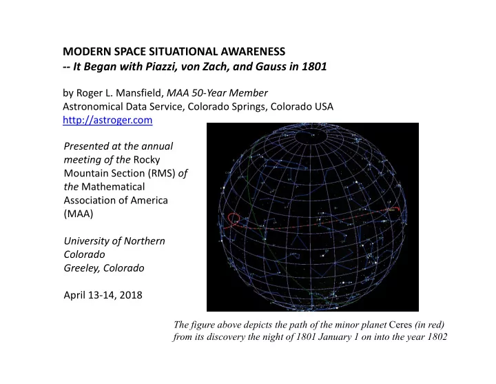
MODERN SPACE SITUATIONAL AWARENESS It Began with Piazzi, von Zach, and Gauss in 1801 by Roger L. Mansfield, MAA 50 Year Member Astronomical Data Service, Colorado Springs, Colorado USA http://astroger.com Presented at the annual meeting


slide-1
SLIDE 1

MODERN SPACE SITUATIONAL AWARENESS ‐‐ It Began with Piazzi, von Zach, and Gauss in 1801

by Roger L. Mansfield, MAA 50‐Year Member Astronomical Data Service, Colorado Springs, Colorado USA http://astroger.com Presented at the annual meeting of the Rocky Mountain Section (RMS) of the Mathematical Association of America (MAA) University of Northern Colorado Greeley, Colorado April 13‐14, 2018

The figure above depicts the path of the minor planet Ceres (in red) from its discovery the night of 1801 January 1 on into the year 1802

slide-2
SLIDE 2

Space Situational Awareness - Now

2

  • The U.S. Air Force operates a global network of radar and

electro‐optical sensors

  • These sensors detect and track artificial Earth satellites
  • The electro‐optical sensors collect observations consisting
  • f time, right ascension (RA), and declination (DEC)
  • These observations go to the Joint Space Operations

Center (JSpOC) at Vandenberg Air Force Base

  • Using these observations, the JSpOC maintains a catalog of

all deep‐space objects in Earth orbit larger than about 10 cm

– A deep‐space object has a mean orbital motion of less than 6.4

  • rbital revolutions per day, whereas a near‐Earth object has a

mean orbital motion of 6.4 orbital revolutions per day or more

  • Next slide is Fig. 1 ‐ Handout Map of the Celestial Sphere
slide-3
SLIDE 3
slide-4
SLIDE 4

Space Situational Awareness - Now

4

  • The handout map depicts the entire celestial sphere

– RA ranges from 0 to 360 degrees (0‐24 hours) and DEC ranges from ‐90 degrees to +90 degrees

  • So every observation made by an electro‐optical sensor

can be plotted on this map

  • The purpose of the Air Force's space catalog is to facilitate

space situational awareness, i.e., ‐ what is up there in space? ‐ what is it doing there?

  • You can access this space catalog by going to

http://space-track.org and creating an account

see also http://celestrak.com

slide-5
SLIDE 5

Space Situational Awareness - 1801

5

  • In 1801, the Italian mathematician and astronomer

Giuseppe Piazzi was observing the night sky

– using the highly‐precise Palermo (Sicily) meridian circle telescope

  • Piazzi's objective was to measure the right ascensions and

declinations of stars, in order to compile a star catalog

  • But Piazzi found a hitherto‐unknown object that was

moving slowly from night to night

– Astronomers of the day, e.g., Baron Franz Xaver von Zach, thought that there might be an undiscovered major planet between Mars and Jupiter. Was this was it?

  • Slide 6 depicts Piazzi’s observations

– 19 complete observations taken from the night of 1801 January 1 to 1801 February 11, as published by von Zach in his Monatliche Correspondenz (MC) for September 1801

  • Slide 7 depicts actual path of Ceres on celestial sphere
slide-6
SLIDE 6

Space Situational Awareness - 1801

6

Figure 2. Piazzi’s observations of the unknown celestial object (Ceres)

slide-7
SLIDE 7

Figure 3. Path of Ceres from discovery in the constellation Taurus to recovery in the constellation Leo

7

The figure is an

  • rthographic pro‐

jection of the celestial

  • sphere. 60 points of

the ephemeris of Ceres are plotted at 10‐day intervals. Note that the path of Ceres looped in the tail of Leo. Ceres was recovered, using the Gauss search ephemeris, as it entered the loop. *Software Bisque’s TheSky program was used here – see

http://bisque.com

*

slide-8
SLIDE 8

Space Situational Awareness - 1801

8

  • The new celestial object was of great interest, but was lost

from observation for almost the entire year 1801

  • Carl Friedrich Gauss, mathematician, mathematical

physicist, and astronomer took note of these observations and computed an orbit for the object

  • Gauss's orbit put the object on a heliocentric path

between the orbits of Mars and Jupiter

  • Next slide shows Gauss's search ephemeris, as published

by von Zach in the December 1801 issue of Monatliche Correspondenz

slide-9
SLIDE 9

Search Ephemeris of Gauss from Monatliche Correspondenz,

  • Vol. 4, p. 647:

Table 4, Page 11 of my AMOS 2016 paper

converts Gauss’s geocentric ecliptic longitudes and latitudes to right ascensions and declinations* *Using formulas in Chapter IV of William Marshall Smart’s, Text‐ Book on Spherical Astronomy, 5th edition (Cambridge University Press, 1965), p. 40. Z column contains “Zodiac Number” 0 through 11, to be multiplied by 30 degrees and added to degrees column

Gregorian Date Ecliptic Longitude Ecliptic Latitude Right Ascension Declina- tion year mo da deg mn deg mn hours degrees 1801 11 25 170 16 09 25 11.6558 12.5032 1801 12 01 172 15 09 48 11.7885 12.0665 1801 12 07 174 07 10 12 11.9141 11.6897 1801 12 13 175 51 10 37 12.0316 11.3805 1801 12 19 177 27 11 04 12.1417 11.1550 1801 12 25 178 53 11 32 12.2418 11.0116 1801 12 31 180 10 12 01 12.3331 10.9438

Space Situational Awareness - 1801

9

Figure 4. Conversion of the geocentric ecliptic longitudes and latitudes in Gauss’s search ephemeris (table on left) to right ascensions and declinations (table on right)

slide-10
SLIDE 10

Space Situational Awareness - 1801

10

  • Using Gauss’s search ephemeris, von Zach observed (recovered)

the new object on the night of 1801 December 31 ‐ 1802 January 1

  • Gauss became a "celebrity" throughout Europe as the result of

his ingenious and extremely difficult feat of mathematical computation (with quill pen, ink, paper, and log tables!)

  • Gauss had devised a method of orbit determination that was

not only novel, but also of enduring interest

  • See Teets and Whitehead (Mathematics Magazine, April 1999)

for an award‐winning, contemporary article that provides a historical sketch and a summary of Gauss's method:

https://www.maa.org/programs/maa-awards/writing-awards/the-discovery-of-ceres-how-gauss-became-famous

slide-11
SLIDE 11

Motivation and Background

11

  • Became interested in the discovery of Ceres because of a project

I was doing with Dr. Gim J. Der, whose MIT Ph.D. dissertation advisor was the great astrodynamicist Richard H. Battin (1925‐ 2014)

  • Dr. Battin was chief architect of the guidance and control

hardware and software for the Apollo missions to the Moon

  • Go to this link for an oral history of Dr. Battin’s career:

https://www.jsc.nasa.gov/history/oral_histories/BattinRH/BattinRH_4-18-00.htm

  • Dr. Der and I wanted to apply some of the algorithms that we

had developed for modern space situational awareness to Piazzi’s observations

  • We also wanted to compare our results with Gauss's results, if

possible

slide-12
SLIDE 12

Difficulties, Rewards, and Results of My Research

12

  • Was surprised and pleased to find that a public domain

reprint of von Zach's Monatliche Correspondenz articles from 1801 had become available in the U.S. (since 2012)

  • But my historical research was difficult, because von Zach's

articles were

– in German (not my native tongue, but studied in college) – early nineteenth‐century German, at that – and the printed copy available to me was/is of rather poor quality

  • Had not been aware that Gauss‘s search ephemeris had

been published by von Zach

– This was exactly what I needed to validate my own results

  • Next slide depicts my results graphically
slide-13
SLIDE 13

Comparison of Contemporary vs. 1801 Results

13

Figure 5. Comparison of Contemporary Results with Gauss Search Ephemeris

  • Red curve in Fig. 5 is the contemporary JPL Horizons‐computed path of Ceres for

times during 1801‐1802 (best available modern ephemeris)

  • Green curve is through seven points plotted from Gauss’s search ephemeris
  • Black curve is through the seven points computed from my own determination

and differential correction of the orbit of Ceres from Piazzi’s observations

  • My "statistically valid" orbit for Ceres,
  • btained from 17 good Piazzi observations
  • ut of 19 possible, was not as good as

Gauss's orbit

  • But my orbit as depicted in Fig. 5, using

the exact same three observations that Gauss used, was slightly better than Gauss's orbit

  • I attribute the improvement to my having

a better solar ephemeris in 2016 than was available to Gauss in 1801

slide-14
SLIDE 14

Summary of this MAA/RMS 2018 Presentation

14

  • In 1801, astronomers were scanning the skies with telescopes,

compiling star catalogs, and looking for new objects in orbit around the Sun

  • Today, the Air Force scans the skies with telescopes ‐‐ and with

radars as well ‐‐ looking for new objects in orbit around Earth

  • Piazzi, von Zach, and Gauss pioneered in 1801 the methods and
  • perational techniques of modern space situational awareness

– because Gauss devised a new method of orbit determination still now in use, ‐ for space objects in orbit around the Sun ‐ for space objects detected in orbit around Earth – and because we use our modern, highly‐precise star catalogs ‐ to discriminate the unknown from the familiar, as Piazzi did, ‐ and to make our observations more accurate

slide-15
SLIDE 15

References

15

[1] von Zach, Franz Xaver, Monatliche Correspondenz zur Befoerderung der Erd‐ und Himmelskunde, Vol. 4 (1801). Search for the book likely only at Amazon.com, then:

[a] Piazzi’s observations ‐ September 1801 (p. 280) [b] Gauss’s search ephemeris for Ceres ‐ December 1801 (p. 647)

[2] Mansfield, Roger L. and Gim J. Der, “Reconstruction of the 1801 Discovery Orbit of Ceres via Contemporary Angles‐Only Algorithms,” Advanced Maui Optical and Space Surveillance Technologies (AMOS) Conference 2016, Maui, Hawaii, September 20‐23, 2016.

http://astroger.com/Mansfield_Der_AMOS_2016_09_15_preprint.pdf

slide-16
SLIDE 16

Addenda (Time Permitting)

16

  • How to use the handout star chart (Fig. 1, p. 3)

– The celestial meridian is fixed at any observer’s (e.g., your) longitude and extends from celestial north pole to celestial south pole

  • The celestial meridian can be depicted on the map as a vertical line from the upper

border of the map to its lower border

– You can simulate the celestial meridian with a pen placed on the map in vertical orientation

  • Place pen at the point on the map corresponding to tonight’s date. This is the

location of the celestial meridian at midnight tonight

  • Move pen one hour to the right for each hour earlier than midnight
  • Move pen one hour to the left for each hour later than midnight
  • The celestial meridian now tells you which constellations you will see above your

local horizon as you look due south

– See the third link at http://astroger.com for more details

  • Next slide provides an overview of the Mathcad PRIME 4.0

worksheet used to convert geocentric ecliptic longitudes and latitudes of Ceres to right ascensions and declinations

slide-17
SLIDE 17

Addenda (Time Permitting)

17

  • Conversion of geocentric ecliptic longitudes and latitudes to right ascensions and

declinations – Let Lambda be geocentric ecliptic longitude and let Beta be geocentric ecliptic latitude – Let Alpha be right ascension and let Delta be declination – Let ε be the obliquity of the ecliptic and let JDT be the Julian date – Then a Mathcad function that does the calculations is: See the Mathcad PRIME 4.0 worksheet at http://astroger.com for further details.

slide-18
SLIDE 18

Appendix – Two More Star Maps

18

  • The rectangular projection on p. 3 of this presentation is not a conformal

mapping of the celestial sphere to the plane

– But it does highlight the ecliptic path of the Sun and the twelve Zodiac constellations spread out along the ecliptic – At the expense of greatly distorting the star regions around the north and south celestial poles

  • The next two slides contain two more maps:

– Polar equidistant projection of the north celestial hemisphere down to ‐45 degrees declination – Polar equidistant projection of the south celestial hemisphere up to +45 degrees declination

  • So the two maps cover the entire celestial sphere, with 90 degrees of
  • verlap, i.e.,

– The first map extends 45 degrees into the southern hemisphere – The second map extends 45 degrees into the northern hemisphere

  • And they display the north and south polar regions in the manner that

we would expect to observe them

slide-19
SLIDE 19
slide-20
SLIDE 20