model selection information criteria akaike information
play

Model Selection & Information Criteria: Akaike Information - PDF document

CS 109A: A dvanced T opics in D ata S cience P rotopapas , R ader Model Selection & Information Criteria: Akaike Information Criterion A uthors : M. M attheakis , P. P rotopapas 1 Maximum Likelihood Estimation In data analysis the


  1. CS 109A: A dvanced T opics in D ata S cience P rotopapas , R ader Model Selection & Information Criteria: Akaike Information Criterion A uthors : M. M attheakis , P. P rotopapas 1 Maximum Likelihood Estimation In data analysis the statistical characterization of a data sample is usually performed through a parametric probability distribution (or mass function ), where we use a distribution to fit our data. The reason that we want to fit a distribution to our data is that it is easier to work with a model rather than data, and it is also more general. There are a lot of types of distributions for di ff erent types of data. Examples include, Normal, exponential, Poisson, 
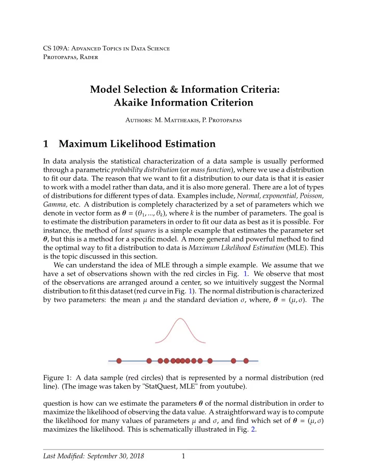
Gamma, etc. A distribution is completely characterized by a set of parameters which we denote in vector form as θ = ( θ 1 , ..., θ k ), where k is the number of parameters. The goal is to estimate the distribution parameters in order to fit our data as best as it is possible. For instance, the method of least squares is a simple example that estimates the parameter set θ , but this is a method for a specific model. A more general and powerful method to find the optimal way to fit a distribution to data is Maximum Likelihood Estimation (MLE). This is the topic discussed in this section. We can understand the idea of MLE through a simple example. We assume that we have a set of observations shown with the red circles in Fig. 1. We observe that most of the observations are arranged around a center, so we intuitively suggest the Normal distribution to fit this dataset (red curve in Fig. 1). The normal distribution is characterized by two parameters: the mean µ and the standard deviation σ , where, θ = ( µ, σ ). The Figure 1: A data sample (red circles) that is represented by a normal distribution (red line). (The image was taken by "StatQuest, MLE" from youtube). question is how can we estimate the parameters θ of the normal distribution in order to maximize the likelihood of observing the data value. A straightforward way is to compute the likelihood for many values of parameters µ and σ , and find which set of θ = ( µ, σ ) maximizes the likelihood. This is schematically illustrated in Fig. 2. Last Modified: September 30, 2018 1

  2. Figure 2: Maximum Likelihood Estimation (MLE): Scanning over the parameters µ and σ until the maximum value of likelihood is obtained. (The images were taken by "StatQuest, MLE" from youtube). A formal method for estimating the optimal distribution parameters θ is given by the MLE approach. Let us describe the main idea behind the MLE. We assume, conditional on θ , a parametric distribution q ( y | θ ), where y = ( y 1 , ..., y n ) T is a vector that contains n measurements (or observations). The likelihood is defined by the product: n � q ( y i | θ ) , L ( θ ) = (1) i = 1 and gives a measure of how likely it is to observe the values of y given the parameters θ . Maximum likelihood fitting consists of choosing the distribution parameters θ that maximizes the L for a given set of observations y . It is easier and numerically more stable to work with the log-likelihood, since the product turns to summation as follows n log � q ( y i | θ ) � , � ℓ ( θ ) = (2) i = 1 where log here is the natural logarithm. In MLE we are able to use log-likelihood ℓ instead of the likelihood L because their derivatives become zero at the same point, since ∂ θ = ∂ ∂ℓ ∂ θ log L = 1 ∂ L ∂ θ , L hence, both L ( θ ) and ℓ ( θ ) become maximum for the same set of parameters θ , which we will call θ MLE , and thus, ∂ � = ∂ � � � ∂ θ ℓ ( θ ) = 0 . ∂ θ L ( θ ) � � � � � θ = θ MLE � θ = θ MLE We present the basic idea of the MLE method through a particular distribution, the exponential. Afterwards, we present a very popular and useful workhorse algorithm that is based on MLE, the Linear Regression model with normal error . In this model, the optimal distribution parameters that maximize the likelihood can be calculated exactly (analytically). Unfortunately, for most distributions the analytic solution is not possible, so we use iterative methods (such as gradient descent) to estimate the parameters. Last Modified: September 30, 2018 2

  3. 1.1 Exponential Distribution In this section, we describe the Maximum Likelihood Estimation (MLE) method by using the exponential distribution . The exponential distribution occurs naturally in many real-world situations such as economic growth, the increasing growth rate of microorganisms, virus spreading, the waiting times between events (e.g. views of a streaming video in youtube), in nuclear chain reactions rates, in computer processing power (Moore’s law), and in many other examples. Consequently, it is a very useful distribution. The exponential distribution is characterized by just one parameter, the so-called rate parameter λ , which is proportional to how quickly events happen, hence θ = λ . Considering that we have n observations that are given by the vector y = ( y 1 , ..., y n ) T , and assuming that these data follow the exponential distribution, then they can be described by the exponential probability density: � λ e − λ y i y i ≥ 0 f ( y i | λ ) = y i < 0 . (3) 0 The log-likelihood that corresponds to the exponential distribution density (3) is deter- mined by the formula (2) and given by n n � . � � � λ e − λ y i � ℓ ( λ ) = log = � log ( λ ) − λ y i (4) i = 1 i = 1 Since we have only one distribution parameter ( λ ), we are maximizing the log-likelihood (4) with respect to λ , hence n ∂λ = n ∂ℓ � λ − y i = 0 , i = 1 where the solution estimates the optimal parameter λ MLE that maximizes the likelihood to be: − 1 n   1 �   λ MLE = y i . (5)      n    i = 1 Inspecting the expression (5) we can observe that λ MLE is the inverse of the mean of our data sample. This is a useful property of the rate parameter. 1.2 Linear Regression Model Linear regression is a workhorse algorithm that is used in many scientific fields such as finance, the social sciences, the natural sciences and data science. We assume a dataset with n training data-points ( y i , x i ), for i = 1 , ..., n , where y i accounts to the i -th observation for the input point x i . The goal of the linear regression model is to find a linear relationship between the quantitative response y = ( y 1 , ..., y n ) T on the basis of the input (predictor) vector x = ( x 1 , ..., x n ) T . In Fig. 3 we illustrate the probabilistic interpretation of linear regression and the idea behind the MLE for linear regression model. In particular, we show a sample set of points ( y i , x i ) (red filled circles), and the corresponding prediction of Last Modified: September 30, 2018 3

  4. Figure 3: Linear regression model. The red filled circles show the data points ( y i , x i ) while the red solid line is the prediction of linear regression model. the linear regression model at the same x i (solid red line). We obtain the best linear model when the total deviation between the real y i and the predicted values is minimized. This is achieved by maximizing the likelihood. As a result we can use the MLE approach. The fundamental assumption of the linear regression model is that each y i is normally (gaussian) distributed with variance σ 2 and with mean µ i = β · x i = x T i β , hence k � x ij β j + ǫ i y i = j = 0 = x i · β + ǫ i = x T i β + ǫ i , where ǫ i is a gaussian random error term (or white stochastic noise) with zero mean and variance σ 2 , i.e. ǫ i ∼ N ( ǫ i | 0 , σ 2 ), k is the size of the coe ffi cient vector β and now each x i is a vector of the same size k ; this statement is graphically demonstrated by the black gaussian curves in Fig. 3. The observation y i is assumed to be given by the conditional normal distribution y i = q ( y i | µ i , σ 2 ) = N ( y i | µ i , σ 2 ) = N ( y i | x T i β , σ 2 ) (6) ( y i − x T i β ) 2 � � 1 = 2 πσ 2 exp − . (7) √ 2 σ 2 Using the formulas (1) and (2) we write the likelihood for the normal distribution (6) as n ( y i − x T i β ) 2 � � 1 � L ( β , σ 2 ) = 2 πσ 2 exp − , (8) √ 2 σ 2 i = 1 Last Modified: September 30, 2018 4

Download Presentation
Download Policy: The content available on the website is offered to you 'AS IS' for your personal information and use only. It cannot be commercialized, licensed, or distributed on other websites without prior consent from the author. To download a presentation, simply click this link. If you encounter any difficulties during the download process, it's possible that the publisher has removed the file from their server.

Recommend


More recommend