Model inference s e from l b a v observed data r e s b o - - PowerPoint PPT Presentation

model inference
SMART_READER_LITE
LIVE PREVIEW

Model inference s e from l b a v observed data r e s b o - - PowerPoint PPT Presentation

Model inference s e from l b a v observed data r e s b o time dynamics underlying mechanisms predictive model (correlations) (interactions) Many issues : limitation over temporal and spatial sampling, noise (measurement,


slide-1
SLIDE 1

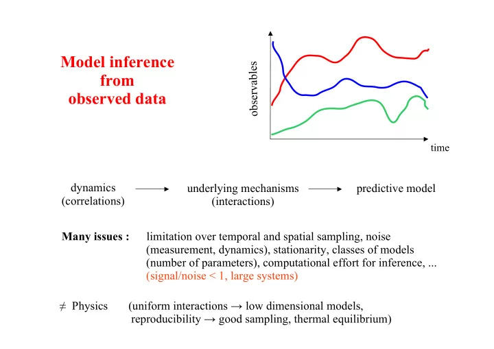
Model inference from

  • bserved data

time

dynamics (correlations) underlying mechanisms (interactions)

  • b

s e r v a b l e s predictive model Many issues : limitation over temporal and spatial sampling, noise (measurement, dynamics), stationarity, classes of models (number of parameters), computational effort for inference, ... (signal/noise < 1, large systems) ! Physics (uniform interactions " low dimensional models, reproducibility " good sampling, thermal equilibrium)

slide-2
SLIDE 2

Example 1:

Concerted activity of a neural population

Fujisawa, Amarasingham, Harrison, Buzsaki (2008) Schnitzer, Meister (2003) Schneidman et al. (2006)
slide-3
SLIDE 3
  • Network depend on activity (functional connections)
  • Connections can be modified through learning …
  • More sophisticated methods to infer effective connections for encoding/decoding:

input

  • utput

encoding decoding

! Talk by S. Cocco on replay of cell assemblies after learning (memory consolidation)

slide-4
SLIDE 4

Example 2:

Coevolution of residues in protein families

Morais Cabral et al. (1996)

PDZ domains

Gobel et al. (1994)
  • Conservation of residues (used for homology detection, phylogeny reconstruction)
  • Two-residue correlations ? could reflect structural and functional constraints ...

! Talk by M. Weigt on covariation in protein families and the inverse Hopfield model ! Talk by O. Rivoire on spin glass models for protein evolution

slide-5
SLIDE 5

Example 3:

Order and organization in bird flocks

! Talk by by A. Jelic on information transfer in flocks of starlings

slide-6
SLIDE 6

Issues : Measurement noise, dynamical noise, limited number of samples, unknown (not measured) species, … Is there any reliable signal about species-species 'interactions'? (additivity?) Exploit interactions to predict dynamics, extinction ? dNi dt = Ni ( ri – # Aij Nj ) Lotka-Volterra equations:

j

Example 4:

Coupled dynamics of species in an ecological system

Population ecology : interactions between species (existence, additivity, …)

slide-7
SLIDE 7

Goals

  • Compression of data (eliminate indirect correlations, sparser representation?)
  • Find effective interaction network

(ex: contact map in protein residue case)

  • Obtain predictive, generative models

(ex : model for artificial protein sequences)

  • Feedback with experiments : design of optimal, maximally informative

protocols

Could be used to test effect of perturbation … to define 'energy' landscape and probe configuration space ...

correlated activity interaction interaction interaction
slide-8
SLIDE 8

Microscopic model for the data (1)

mi = <!i >, cij = <!i$j >, ... (constraints are realizable) Constraints Data

(1,0,0,0,1,0,1,1, ..., 1,0,0,1,1,0) (0,1,0,0,0,1,1,1, ..., 0,1,1,0,0,0) (1,1,0,1,0,1,1,0, ..., 1,1,0,0,1,1) ... (0,1,0,0,1,0,0,0, ..., 0,0,0,1,0,0)

" Probability p($1, $2 ,... , $N )? Maximum entropy principle (Jaynes, 1957)

Find p(!) maximizing the entropy S[p] = - % p(!) ln p(!) under the selected constraints ! (here, stationary and discrete data)

slide-9
SLIDE 9

Microscopic model for the data (2)

Analogy with Thermodynamics and Ensembles in Statistical Physics

  • System with energy E, volume V, N particles, ...
  • Fix average value of volume V # impose pressure p : E $ E + pV

number of particules N # impose chemical potential µ : E $ E - µ N Model

  • E(!;J,h) = - ! Jij $i $j - ! hi $i
  • pMAXENT(!;J,h) = exp( -E(!;J,h) ) / Z[J,h]

where Z[J,h] = % exp( -E(!;J,h) )

  • find couplings and fields such that all N+ N(N-1)/2 constraints are fulfilled
i<j i

Ising model! ! & ln Z[J,h] & hi = mi & ln Z[J,h] & Jij = cij

,

slide-10
SLIDE 10

Boltzmann Machine Learning

  • Start from random Jij and hi
  • Calculate <$i$j> and <$k> using Monte Carlo simulations
  • Compare to cij and mk (data) and update Jij $ Jij - a (<$i$j> - cij) )

hk $ hk - a (<$k> - mk) Problems:

  • 1. issue of thermalization (critical point ?

may take exponential-in-N time …)

  • 2. convergence (yes, but flat modes ?)

$ slow

Ackley, Hinton, Sejnowski (1985)
slide-11
SLIDE 11

Microscopic model for the data (3)

Cross-entropy of data (= !1,...,!B ) S† [J,h] = % - ln p(!b;J,h) = B ( ln Z[J,h] - ! Jij cij - ! hi mi )

b=1 B i<j i

J,h S†[J,h;data]

  • The minimum of S is the Ising model we are looking for :
  • The Hessian of S is positive semi-definite, hence S is convex

J*,h* S[p] S[pMAXENT] = S† [J*,h*] S† [J,h]

slide-12
SLIDE 12

Microscopic model for the data (4)

Hessian of the cross-entropy &2 S(J,h;data) & (J,h) & (J,h)

=

<$i$j$k$l> - <$i$j> <$k$l> <$i$j$k> - <$i$j> <$k> <$i$j> - <$i> <$j>

( )

<$i$j$k> - <$i> <$j$k>

XT ( ) X = (# xij ($i$j- <$i$j>) + # xk ($k- <$k>))2 ( ) xk xij X =

< >

i<j k

$

where < > = Gibbs average with the Ising model

Zero modes ? Log-prior on the parameters...

J,h

slide-13
SLIDE 13

Bayesian inference framework (1)

Data = set of configurations !b , b = 1, 2, … , B= nb. of configs

P[ ! | J,h ] = exp( ! Jij $i $j + ! hi $i) / Z[J,h]

b i<j i

P0[ J,h ] (useful in case of undersampling ...)

Bayes formula

P[ J,h | Data] ' & P[ !b | J,h ] ( P0[ J,h ]

Likelihood Prior

For instance : P0 ' exp( - ! Jij /(2J2 ))

i<j
slide-14
SLIDE 14

Bayesian inference framework (2)

Regularized Cross-entropy Posterior Proba

  • f J,h

P[ J,h | Data ] ' exp( B[ ! Jij cij + ! hi mi]) / Z[J,h]B

i<j i

' P0[ J,h ] S = - ln P[ J,h | Data ]

i<j i

= B ( ln Z[J,h] - ! Jij cij - ! hi mi ) - ln P0[ J,h ]

i<j i

= B ( ln Z[J,h] - ! Jij cij - ! hi mi ) + ! Jij /(2J2 )

i<j

(with Gaussian prior)

slide-15
SLIDE 15

Questions

  • 1. Practical methods to find interactions Jij from the correlations cij?

(fast, accurate algorithms)

  • 2. How much data does one need to get reliable interactions?

(overfitting ...)

J* $ configurations {Si} $ c $ J |J* ) J|

B = nb. configs

?

slide-16
SLIDE 16

Questions

  • 3. How large should be the sampled sub-system?
correlation length

Is the inverse problem well-behaved ? Asymptotic inference : B $ infinity, while N is kept fixed Error on each parameter of the order of B-1/2 What happens in practice, i.e. when B and N are of the same order of magnitude ?

slide-17
SLIDE 17

Inference approaches

  • Gaussian inference (and Mean field)
  • Inverse Hopfield-Potts model
  • Pseudo-likelihood algorithms
  • Advanced statistical physics methods
slide-18
SLIDE 18

Interactions from correlations for Gaussian variables

N Gaussian variables xi with variances cii = <xixi> = 1 i!j : cij = <xixj> = + + + … Matrix notation: c = Id + J + J2 + J3 + … = (Id-J)-1 " J = Id – c-1 Time = N3

Jij % Jik Jkj

k

% Jik Jkl Jlj

k,l

Problems:

  • Matrix c corrupted by noise, which makes inversion very unreliable

Empirical matrix c = ( )

  • nb. of data

^ cij ± B-1/2 N " Errors of order (N/B)1/2 …

slide-19
SLIDE 19
  • Not correct for discrete variables (neurons=0,1 ; amino-acids=1,2, .., 21)
  • Gaussian theory corresponds to mean-field theory

Why? MF exact when effective fields average out = with many neighbors & weak interactions, and fluctuations are described by Gaussian law example: very large dimensions D in physical systems lead to N(0,1/D)

JGaussian

2-spin system

… but with regularization pseudo-count L2 (quadratic log-prior)

slide-20
SLIDE 20

Inference approaches

  • Mean field inference
  • Inverse Hopfield-Potts model
  • Pseudo-likelihood algorithms
  • Advanced statistical physics methods
slide-21
SLIDE 21

Inverse Hopfield model : retarded learning phase transition

Example: N=100, ! = Gaussian (0,.7) Retarded learning: Watkin, Nadal (1994) Baik, Ben Arous, Peche (2005) #config=40 #config=400

Phase transition! |*+ ) *|

# config / N

slide-22
SLIDE 22

Inverse Hopfield Model : posterior entropy of patterns

Example : P=1 pattern, no field

Retarded learning transition

Cocco, M., Sessak (2011)

( b i t s ) ( b i t s ) ~1/( ?

("c=2, !L =1)

*2/N = 1.1 *2/N = 0.5

slide-23
SLIDE 23

Inverse Hopfield Model : error on the inferred patterns

For pattern components ~1, corrections to S0 are useless (at best) unless many configurations are available ... " Mean-Field is better (even if wrong) when few data are available

slide-24
SLIDE 24

Inference approaches

  • Mean field inference
  • Inverse Hopfield-Potts model
  • Pseudo-likelihood algorithms
  • Advanced statistical physics methods
slide-25
SLIDE 25

Pseudo-likelihood methods (1)

Idea: avoid calculation of partition function using Callen identities (1963)

< $0 > = < tanh( % J0k $k + h0) >

) % tanh( % J0k $k + h0) / B

k J0k

k!0 k!0 b sampled configurations

Pseudo cross entropy:

« S » = % log 2 cosh( % J0k $k + h0) - B (h0m0 + % J0k c0k)

b k!0 k!0 sampled configurations

cost function ({J}) = pseudo-cross entropy (h0,{J0k}) + * % |J0k|

k

Prior: increase signal/noise ratio by exploiting the sparsity of Jij

slide-26
SLIDE 26

Pseudo-likelihood methods (2)

k Jk0

Complexity: if B > a logN, the procedure finds couplings of amplitude |J| > a’ (logN /B)1/2 in time poly(B,N) [a & a’ depend on maximal degree (number of neighbours of i with nonzero Jij)]

  • Ising model should be the true model for data
  • Coupling matrix is not symmetric (but is asymptotically consistent)
  • Susceptibility , should be small (fails in the vicinity of the critical point)
  • All poly algorithms fail at critical point ?

Caveat:

k Jk0

*

cost

Bento, Montanari (2009) Ravikumar, Wainwright, Lafferty (2010)
slide-27
SLIDE 27

What is the relevant susceptibility for the inverse problem?

Susceptibility: ,ij,kl =

+ <si sj > + Jkl

= response of a correlation to a small change in an interaction may be long range ...

J

Susceptibility: ,ij,kl =

+ <sk sl > + Jij

= response of an interaction to a small change in a correlation Inverse

  • 1

<ss > Jij

  • ckl
  • ckl

Inverse problem is well-behaved if ,)1 short range !

slide-28
SLIDE 28

Examples of inverse susceptibility matrices

  • Spherical (Gaussian) models : ,)1
ij,kl = JikJjl has the same sparsity as J
  • Liquid theory: ,)1 is closely related to the Ornstein-Zernike

direct correlation function. The short-rangedness of ,)1

is used for closure scheme e.g. Percus-Yevick
  • Critical point of ferromagnet: ,)1(q) ~ q2--

hence, ,r>R dr ,)1(r) decays with R

  • 1D Ising model : 4-point ,)1 is sparse!
  • Real data?

R

slide-29
SLIDE 29

Inference approaches

  • Mean field inference
  • Inverse Hopfield-Potts model
  • Pseudo-likelihood algorithms
  • Advanced statistical physics methods
slide-30
SLIDE 30

Adaptive cluster expansion (1)

= % *S. (mi) + % *S./ (mi,mj,cij) + % *S./0 (mi,mj,mk,cij,cik,cjk) + ...

Cross-entropy

S = min - % log P(s1,s2,...,sN|J,h)

J,h

sampled configurations i i<j i<j<k

cij mj mi mi

" hi " 1hi , 1hi , Jij

cij mj mi mk cik ckj

" 11hi , 11hi , 1Jij (and other variables...)

Cocco, R.M. (2011,2012) ; Barton, Cocco (2012)
slide-31
SLIDE 31

Adaptive cluster expansion (2)

Large cluster entropies are network-specific Small cluster entropies are due to sampling noise

cij |i-j|

#config-1/2

slide-32
SLIDE 32

Adaptive cluster expansion (3)

  • Number & size of clusters adapt to data structure
  • J is (almost surely) unveiled if B >> log N (and not N)
  • Successful on critical Ising models in 2D
Universal distribution (independent spins)
slide-33
SLIDE 33

Application to retinal recordings (1)

N=32-60 ganglion cells recorded for about 2000 sec (spontaneous activity)

Meister et al. (2003)

2m

mi

Schneidmann et al., Nature (2006) Shlens et al., J. Neuroscience (2006)

retina visual stimulus MEA

slide-34
SLIDE 34

Application to retinal recordings (2)

Maps in retinal plane

Cocco, M., Leibler (2009)
slide-35
SLIDE 35

Is the Ising model good? (1)

Ability to predict higher order moments: Schneidmann et al., Nature (2006)

Qualitatively good also for very rare configurations = unobserved in recording …!

slide-36
SLIDE 36

Is the Ising model good? (2)

S1 > S2 > S3 > ...> SN

SK = entropy with moments of order

L- K imposed ( S

1
  • S
2

) / ( S

1
  • S
N

)

slide-37
SLIDE 37

Is the Ising model good? (3)

But …

S1 > S2 > S3 > ...> SN

SK = entropy with moments of order

L- K imposed ( S

1
  • S
2

) / ( S

1
  • S
N

)

slide-38
SLIDE 38

Is the Ising model good? (4)

Evidence that 2nd moments are not sufficient in some cases:

  • J. Victor et al. (3-body moments),
  • G. Tkakic et al. (P(k))

General understanding of the underlying reasons for success is lacking:

  • why MEP distribution?
  • how smooth should target distribution be?
  • choice of observables (=constraints)?
slide-39
SLIDE 39

Response to multi-drug combinations in bacteria

Wood, Nishida, Sontag, Cluzel, PNAS (2012)

No simple way to predict response to combination of 2 drugs from responses to single drugs (independent, antagonistic, synergistic) …

slide-40
SLIDE 40

Response to multi-drug combinations in bacteria

But response to combinations of 3 or 4 drugs are predictable from 2- and 1- drug responses!

E-Coli

slide-41
SLIDE 41

Conclusion (2)

  • Quality and quantity of data make microscopic modeling possible
  • Hopfield model offers Ising model with natural prior
  • Difficulty: generative models …
  • See talks this afternoon!