Estimating Recall the general mean-variance specification E( Y | x - - PowerPoint PPT Presentation

ST 762 Nonlinear Statistical Models for Univariate and Multivariate Response

Estimating θ

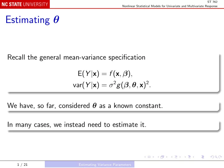
Recall the general mean-variance specification E(Y |x) = f (x, β), var(Y |x) = σ2g(β, θ, x)2. We have, so far, considered θ as a known constant. In many cases, we instead need to estimate it.

1 / 21 Estimating Variance Parameters

ST 762 Nonlinear Statistical Models for Univariate and Multivariate Response

One approach is to continue to use the Gaussian likelihood: −n log σ −

n

• j=1

log g (β, θ, xj) − 1 2

n

• j=1

{Yj − f (xj, β)}2 σ2g (β, θ, xj)2 . Differentiating w.r.t. θ leads to

n

• j=1
• {Yj − f (xj, β)}2 − σ2g (β, θ, xj)2

σ2g (β, θ, xj)2

• νθ (β, θ, xj) = 0.

2 / 21 Estimating Variance Parameters

ST 762 Nonlinear Statistical Models for Univariate and Multivariate Response

Here νθ (β, θ, xj) = ∂ log g (β, θ, xj) ∂θ = gθ (β, θ, xj) g (β, θ, xj) . For consistency with earlier estimating equations, rewrite as

n

• j=1
• {Yj − f (xj, β)}2 − σ2g (β, θ, xj)2

2σ4g (β, θ, xj)4

• 2σ2g (β, θ, xj)2 νθ (β, θ, xj)

= 0.

3 / 21 Estimating Variance Parameters

ST 762 Nonlinear Statistical Models for Univariate and Multivariate Response

Combining with the σ2 equation derived earlier,

n

• j=1
• {Yj − f (xj, β)}2 − σ2g (β, θ, xj)2

2σ4g (β, θ, xj)4

• ×
• 2σg (β, θ, xj)2

2σ2g (β, θ, xj)2 νθ (β, θ, xj)

• = 0.

4 / 21 Estimating Variance Parameters

ST 762 Nonlinear Statistical Models for Univariate and Multivariate Response

The σ2 and θ equations may be put in the standard form

n

• j=1

DT

j V−1 j

(sj − mj) =

((q+1)×1) .

We need sj = {Yj − f (xj, β)}2 mj = σ2g (β, θ, xj)2 Dj =

• 2σg (β, θ, xj)2

2σ2g (β, θ, xj)2 νθ (β, θ, xj) T Vj = 2σ4g (β, θ, xj)4 .

5 / 21 Estimating Variance Parameters

ST 762 Nonlinear Statistical Models for Univariate and Multivariate Response

Since β is also unknown, we must also solve the corresponding equation

n

• j=1

{Yj − f (xj, β)} fβ (xj, β) σ2g (β, θ, xj)2 +

n

• j=1
• {Yj − f (xj, β)}2

σ2g (β, θ, xj)2 − 1

• νβ (β, θ, xj) = 0.

In principle, we must solve the (q + 1) variance parameter equations and the p β equations jointly.

6 / 21 Estimating Variance Parameters

ST 762 Nonlinear Statistical Models for Univariate and Multivariate Response

Joint Estimating Equations Gaussian ML:

n

• j=1

  fβj 2σ2g2

j νβj

2σ2g2

j

1/σ νθj

• 

 σ2g2

j

2σ4g4

j

−1 Yj − fj (Yj − fj)2 − σ2g2

j

• = 0.

GLS:

n

• j=1

  fβj 2σ2g2

j

1/σ νθj

• 

 σ2g2

j

2σ4g4

j

−1 Yj − fj (Yj − fj)2 − σ2g2

j

• = 0.

7 / 21 Estimating Variance Parameters

ST 762 Nonlinear Statistical Models for Univariate and Multivariate Response

Remarks

Solve (p + q + 1) estimating equations jointly. Approach in GLS is called pseudo-likelihood (PL) approach; that is, some parameters are estimated by ML while others are estimated by ad hoc but consistent methods. — GLS-PL When g(·) does not depend on β but does involve unknown θ, νβ (β, θ, xj) = 0, and the normal theory ML and GLS equations coincide.

8 / 21 Estimating Variance Parameters

ST 762 Nonlinear Statistical Models for Univariate and Multivariate Response

Implementation

Write estimating equations in this form, then solve using an idea similar to IRWLS

n

• j=1

DT

j (α)V−1 j (α) {sj(α) − mj(α)} = 0

where DT

j (α) = ∂

∂αmj(α).

9 / 21 Estimating Variance Parameters

ST 762 Nonlinear Statistical Models for Univariate and Multivariate Response

Two strategies Solve the entire set of parameters together: α =   β σ θ   . Iterate between: Given α = σ θ

• , solve for β;

Given β, solve for α.

10 / 21 Estimating Variance Parameters

ST 762 Nonlinear Statistical Models for Univariate and Multivariate Response

Implementation Use Taylor series approximation, α ≈ α∗ +

• DT(α∗)V−1(α∗)D(α∗)

−1 DT(α∗)V−1(α∗) {s(α∗) − m(α∗)} where V(α) = block diag{V1(α), . . . , Vn(α)}, and DT(α) = {DT

1 (α), . . . , DT n (α)}

11 / 21 Estimating Variance Parameters

ST 762 Nonlinear Statistical Models for Univariate and Multivariate Response

Iterative update α(a+1) = α(a) +

• DT

(a)V−1 (a)D(a)

−1 DT

(a)V−1 (a)

• s(a) − m(a)
• Remark: The ML or PL quadratic equations are more unstable than

are the linear equations, and can be ill-behaved in practice.

12 / 21 Estimating Variance Parameters

ST 762 Nonlinear Statistical Models for Univariate and Multivariate Response

A General Class of Estimators of θ

Motivation Estimating equations for θ would be based on the residuals {Yj − f (xj, β)}. For squared residuals, the effect of “outlying” or “unusual”

• bservations can be magnified.

Other functions of the residuals might be considered.

13 / 21 Estimating Variance Parameters

ST 762 Nonlinear Statistical Models for Univariate and Multivariate Response

14 / 21 Estimating Variance Parameters

ST 762 Nonlinear Statistical Models for Univariate and Multivariate Response

Recall The standardized residual: ǫj = Yj − f (xj, β) σg(β, θ, xj) Box-Cox transformation: h(u, λ) =    uλ − 1 λ λ = 0 log |u| λ = 0. Key idea Consider forming estimating equations based on general power transformations of absolute residuals.

15 / 21 Estimating Variance Parameters

ST 762 Nonlinear Statistical Models for Univariate and Multivariate Response

Key assumption The appropriate moments of ǫj are not dependent on xj and are constant for all j: E

• |ǫj|λ

xj

• = E
• |ǫj|λ

= constant ∀j, E

• |ǫj|2λ

xj

• = E
• |ǫj|2λ

= constant ∀j. Definitions Define η such that eλη = σλE(|ǫj|λ) Identify |Yj − f (xj, β)|λ as the “response”.

16 / 21 Estimating Variance Parameters

ST 762 Nonlinear Statistical Models for Univariate and Multivariate Response

It follows that E

• |Yj − f (xj, β)|λ

xj

• = σλg(β, θ, xj)λE
• |ǫj|λ

= eληg(β, θ, xj)λ and var

• |Yj − f (xj, β)|λ

xj

• = σ2λg(β, θ, xj)2λvar
• |ǫj|λ

= σ2λg(β, θ, xj)2λ E

• |ǫj|2λ

− E

• |ǫj|λ2

=

• σ2λE
• |ǫj|2λ

− e2λη g(β, θ, xj)2λ

17 / 21 Estimating Variance Parameters

ST 762 Nonlinear Statistical Models for Univariate and Multivariate Response

Estimating equations

n

• j=1

|Yj − f (xj, β)|λ − eληg(β, θ, xj)λ g(β, θ, xj)2λ

• λeληg(β, θ, xj)λτθ(β, θ, xj) = 0

defines a family of estimating equations for θ, indexed by λ. The quadratic PL equation is obtained when λ = 2.

18 / 21 Estimating Variance Parameters

ST 762 Nonlinear Statistical Models for Univariate and Multivariate Response

Extended quasi-likelihood Recall that quasi-likelihood (QL) was an attempt to give a “distributional” justification for GLS-type estimation of β in models in which the variance depends on β through the mean, but there are no additional, unknown, variance parameters θ (that is, θ is known). When θ is unknown, the idea here is to define a “scaled exponential family-like” “loglikelihood” to be used as a basis for joint estimation

• f β, σ, and θ.

19 / 21 Estimating Variance Parameters

ST 762 Nonlinear Statistical Models for Univariate and Multivariate Response

Recall The log quasi-likelihood function ℓQL(β, σ; y) = 1 σ2 µ

y

y − u g(u)2 du. where µ = f (x, β). Estimate β and σ by maximizing

n

• j=1

ℓQL (β, σ; yj) .

20 / 21 Estimating Variance Parameters

ST 762 Nonlinear Statistical Models for Univariate and Multivariate Response

Define the log extended quasi-likelihood function ℓEQL(β, σ, θ; y) = 1 σ2 µ

y

y − u g(u)2 du − 1 2 log

• 2πσ2g 2(y, θ)
• where µ = f (x, β).

Estimate β, σ, and θ by maximizing

n

• j=1

ℓEQL (β, σ, θ; yj) .

21 / 21 Estimating Variance Parameters