Minimum Earnings Regulation and the Stability of Marketplaces - PowerPoint PPT Presentation

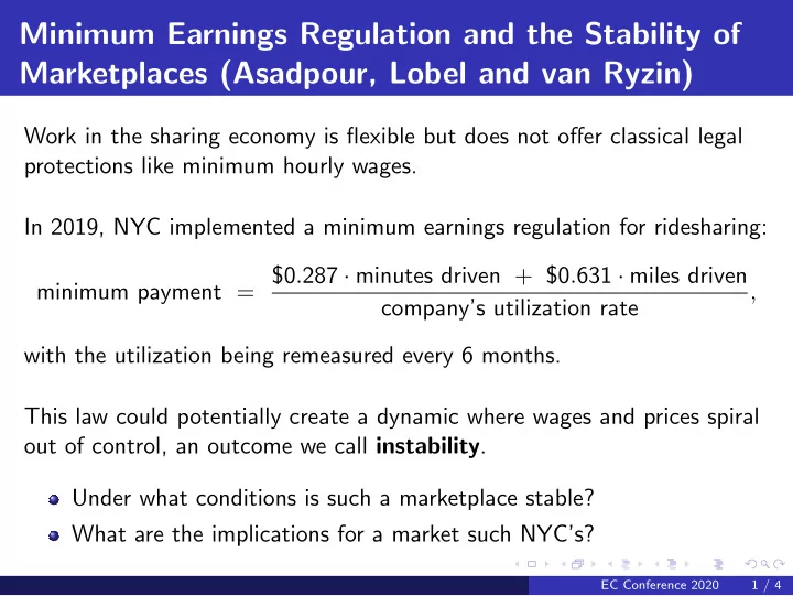
Minimum Earnings Regulation and the Stability of Marketplaces (Asadpour, Lobel and van Ryzin) Work in the sharing economy is flexible but does not offer classical legal protections like minimum hourly wages. In 2019, NYC implemented a minimum earnings regulation for ridesharing: minimum payment = $0 . 287 · minutes driven + $0 . 631 · miles driven , company’s utilization rate with the utilization being remeasured every 6 months. This law could potentially create a dynamic where wages and prices spiral out of control, an outcome we call instability . Under what conditions is such a marketplace stable? What are the implications for a market such NYC’s? EC Conference 2020 1 / 4

The Model A platform sets prices p t and wages w t for each period. Demand is D ( p ) and revenue is R ( p ) � p · D ( p ), with peak p ∗ . Supply is S ( z ) and cost curve is C ( z ) � z · S ( z ). Supply and demand intersect at w ∗ : D ( w ∗ ) = S ( w ∗ ). Supply is a function of earnings z , not wages w . Q ( p , z ) � min { D ( p ) , S ( z ) } : quantity of ride hours produced. u ( p , z ) � Q ( p , z ) / S ( z ): driver utilization. z = w · u ( p , z ): driver earning equilibrium condition . The market is M - minimum-earnings stable if there exists a policy with nonnegative profits in almost all periods where w t +1 ≥ M / u ( p t , z t ) . EC Conference 2020 2 / 4

Main Theorem Inverse cost function: H ( x ) � C − 1 ( x ) C ( z ) = z · S ( z ) Theorem An M-minimum-earnings marketplace is stable if and only if: � p ∗ ≤ w ∗ w ∗ if (tight supply) M ≤ p ∗ > w ∗ H ( R ( p ∗ )) if (loose supply) C ( z ) C ( z ) Total Revenue Total Labor Cost Total Revenue Total Labor Cost R ( p ) R ( p ) H ( R ( p * )) p * w * w * p * stable M Hourly Price Hourly Price Hourly Earning stable M Hourly Earning Loose Labor Supply ( p ∗ ≥ w ∗ ) Tight Labor Supply ( p ∗ < w ∗ ) EC Conference 2020 3 / 4

Calibration Results We use elasticity estimates from the literature to calibrate our model. With w ∗ = $22 . 79 (and net earnings of $14.25), demand elasticity = − 0 . 6, and supply elasticity = 4 . 8: maximum gross earnings = H ( R ( p ∗ )) = $23 . 23 (1 . 9% gain) maximum net earnings = $14 . 69 (3 . 0% gain) Why so little? Because supply is very elastic. C ( z ) Total Revenue Total Labor Cost R ( p ) z = H ( R ( p * )) w * p = w = p * Hourly Price stable M Hourly Earning Ride-hailing providers are likely to remove free-entry from their marketplaces in order to maintain stability. EC Conference 2020 4 / 4