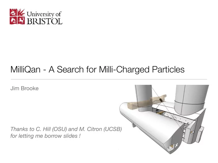
MilliQan - A Search for Milli-Charged Particles Jim Brooke Thanks to - PowerPoint PPT Presentation

MilliQan - A Search for Milli-Charged Particles Jim Brooke Thanks to C. Hill (OSU) and M. Citron (UCSB) ock for letting me borrow slides ! horizontal plane is Clearance to gallery boundaries is ~30

Millikan’s Oil Drop Experiment • Produce charged drops of oil in a chamber • Drops falling at terminal velocity have F drag = F gravity , which allows the radius (and hence mass) to be determined • Apply electric field, such that F grav = F elec = qE, to determine the charge on the drop… � 2

Quantisation of Charge • So electric charge is found in units of e • Or, since the discovery of quarks, units of 1/3 e • Dirac hypothesised a system comprising an electric charge ( e ), and a magnetic monopole ( q m ) • Since angular momentum must be quantised : 2 eq m ∈ Z ~ c • If there is a magnetic monopole, somewhere in the Universe, electric charge must be quantised… � 3

≤ ≤ Monopole Searches 2 eq m • It follows from that the monopole magnetic charge is ∈ Z ~ c q m = ~ c 2 e = e 2 α ∼ 69 e • In terms of ionisation energy loss, a monopole looks like an electrically charged particle with q ~ 69e • Many searches for monopoles that have got stuck in things… � 4

ATLAS Monopole Search [fb] fraction of high threshold track hits 3 ATLAS 10 1.2 HT Events 800 σ DY spin- 1 / ATLAS -1 2 s =8 TeV, 7.0 fb f | | = 1.0 g g 1.1 -1 D 2 s = 8 TeV, 7.0 fb 700 10 = 1000 GeV m 1 600 B A 10 0.9 500 1 0.8 400 DY Spin- 1 / 2 95% CL Limit LO Prediction signal | |=0.5 | |=0.5 g g g g D D 0.7 -1 | |=1.0 | |=1.0 10 g g g g 300 D D | |=1.5 | |=1.5 region g g g g D C D D 0.6 0 500 1000 1500 2000 2500 200 [GeV] m 0.5 100 Data [fb] ATLAS 0.4 2 0 σ 10 -1 s =8 TeV, 7.0 fb 0 0.2 0.4 0.6 0.8 1 1.2 ← cluster dispersion w 10 1 Search for tracks with high dE/dx, DY Spin-0 95% CL Limit LO Prediction associated with narrow EM clusters | |=0.5 | |=0.5 g g g g -1 D D 10 | |=1.0 | |=1.0 g g g g D D | |=1.5 | |=1.5 g g g g D D 0 500 1000 1500 2000 2500 � 5 [GeV] m

MilliCharged Particles • Simple extension to the Standard Model is just to add a U(1) gauge symmetry L = L SM − 1 µ ν − κ B’ B 4 B 0 µ ν B 0 2 B 0 µ ν B µ ν dark SM new ‘dark’ photon kinetic mixing term • Suppose we also have a new fermion, charged only under the new U(1) • Interactions with electric charge can happen via kinetic mixing � 6

Milli-charges • Suppose we add a new fermion, charged only under the new U(1) : L = L SM − 1 0 + im ) ψ − κ ∂ + ie 0 / µ ν + i ¯ 4 B 0 µ ν B 0 2 B 0 µ ν B µ ν ψ ( / A • Then re-define the gauge boson B 0 µ → B 0 µ + κ B µ L = L SM − 1 ∂ + ie 0 / 0 − i κ e 0 / µ ν + i ¯ 4 B 0 µ ν B 0 ψ ( / A B + im ) ψ • The new fermion has a small electric charge, dependent on the kinetic mixing parameter • Call this a milli-charged particle (or mCP) � 7

Existing Constraints on mCPs 0 • Cooling and energy loss from COLL stars & SN LHC E613 - 2 TEX CMB • Degrees of freedom in BBN & SLAC DM - 4 OPOS CMB CMB Neff BBN • Invisible decays of ortho- - 6 Y p Log 10 ( � ) positronium XENON10 SN - 8 • Lamb-shift 1987A Note the • Collider/beam dump searches - 10 Sun big gap ! HB - 12 WD RG - 14 2 4 6 8 10 12 14 Log 10 ( m f / eV ) arXiv:1511.01122 � 8

LHC Results 3 10 × • Searches for tracks with dE/dx 250 Hits -1 CMS, s = 7 TeV, 5.0 fb below that for a q=1 MIP search sample (CMS data) • But tracking is designed for q=1 control sample (CMS data) 200 background simulation modified simulation L (signal simulation) • Sensitivity limited to q>1/3 2/3 L (signal simulation) 1/3 150 5 10 4 10 ) (pb) 100 -1 CMS 5.0 fb at s = 7 TeV 3 10 L q 2/3 L 2 L 10 -1 q 10 1/3 L observed 95% C.L. → 10 50 expected 95% C.L. 1 ± σ (pp expected 95% C.L. 2 ± σ 1 0 1 2 3 4 σ -2 10 q = 1/3 0 2 4 6 8 10 q = 2/3 dE/dx (MeV/cm) -3 10 100 150 200 250 300 350 400 450 500 550 600 m (GeV) L � 9

Improving Sensitivity to low charge • Lower charge -> lower ionisation energy loss • Need a large depth of sensitive material for the particle to traverse • -> increase probability of seeing a hit • Make it su ffi ciently segmented to show the incident particle is compatible with the IP • Look for evidence of ‘tracks’ that have dE/dx lower than that of a q=1 MIP � 10

Proposed Search • Original authors proposed a dedicated experiment Existing Counting Room 1 m • Three-layered scintillator array m 4 . 1 • Background reduced by large amount of rock shielding ψ Existing Wall 20 m • Detect mCP by looking for IP-pointing triple-incidence of low light signals IP • Q=1 will give much bigger signal p p • Backgrounds assumed to arise solely from PMT dark counts 20 m Existing LHC Detector ¯ ψ Haas, Hill, Izaguirre, Yavin PLB 746 (2015) � 11

Proposed Search Haas, Hill, Izaguirre, Yavin PLB 746 (2015) � 12

MilliQan Collaboration • Austin Ball 1 , Jim Brooke 2 , Claudio Campagnari 3 , Albert De Roeck 1 , Brian Francis 4 , Martin Gastal 1 , Frank Golf 3 , Joel Goldstein 2 , Andy Haas 5 , Christopher S. Hill 4 , Jim Hirschauer 10 , Eder Izaguirre 6 , Benjamin Kaplan 5 , Stephen Lowette 12 , Gabriel Magill 7,6 , Bennett Marsh 3 , David Miller 8 , Chris Neu 9 , Theo Prins 1 , Harry Shakeshaft 1 , David Stuart 3 , Max Swiatlowski 8 , Itay Yavin 7,6 , and Haitham Zaraket 11 � 13

Letter Of Intent arXiv:1607.04669 • LOI published in July 2016 • Location identified • Relationship with CMS understood • Full detector simulation • Updated sensitivity � 14

Location, Location, Location • Constraints: • Near LHC P1 or P5 for maximum luminosity • Behind at least 5m of concrete, based on previous tests in CMS counting room • Space to accommodate the detector ~ 1m x 1m x 3m • Floor loading to be compatible with detector and its support structure ~3500kg - 6000kg • Power supply available, with possibility to add other network etc. • Selected experimental area should remain clear of “visitors” during 
 data taking • Many sites near P1 and P5 considered - eventually settled on PX56 � 15

Location, Location, Location • • � 16

Location, Location, Location proposed detector site access PX56 - disused shaft drainage gallery UXC 55 USC 55 ock horizontal plane is Interaction Point Clearance to gallery boundaries is ~30 � 17

Tunnel Survey CERN performed a laser scan of the tunnel Useful in figuring out whether the detector will fit ! 3x1x1 CERN & Lebanese University also designed a support structure that would allow the whole array to be aligned toward the IP � 18

Tunnel Survey • CERN team have extended the CMS t! coordinate system to PX56 • Expect to align MilliQan with ~2cm μ μ precision Center of milliQan goes here! � 19

mCP Production Cross-Section pp → ψ ¯ ψ + X Note the proportionality to q 2 ! � 20

Simulation • Simulate mCP production via Drell-Yan, j/ ψ , Υ . Cross-section ∝ q 2 • Propagate through CMS magnetic field • Simulate interactions with rock, calculate rate of mCP incidence at detector arXiv:1607.04669 � 21

Simulation • Full GEANT4 simulation : reflectivity, attenuation, shape of scintillator. • We input quantum e ffi ciency, scintillator light spectrum, time constants, digitised waveforms Simulation of a single mCP event ⟨ nPE ⟩ = 1 for Q = 0.003e arXiv:1607.04669 � 22

Simulation Efficiency vs Charge 0.1GeV mCP Detector Efficiency 0.1GeV mCP 1 1 0.5 0.100 Efficiency Efficiency ξ = 0.00236 0.010 ξ = 0.00236 0.2 10cm × 10cm r = 0.98 10cm × 10cm r = 0.98 10cm × 10cm r = 0.92 10cm × 10cm r = 0.92 5cm × 5cm r = 0.98 5cm × 5cm r = 0.98 0.001 0.1 0.002 0.004 0.006 0.008 0.010 0.002 0.004 0.006 0.008 0.010 ϵ = Q / e ϵ = Q / e • E ffi ciency to produce > 1PE in a single bar (L) and full detector (R) • Black line is parameterisation used in original paper • Red/blue show GEANT4 results for di ff erent reflectivity/dimensions arXiv:1607.04669 � 23

SPE calibration using LED HV Function Optional cardboard Generator light-blocker e.g. -1450 V 20 ns pulse 2000x filter LED 3D-printed PMT casing to hold LED PMT, LED, filters PMT DRS TRG IN PMT Output (scope) Send simultaneous LED pulse and trigger Digitise and record waveforms Will show results for Measure pulse area example PMT (R878) using integral of window � 24 M. Citron mcitron@ucsb.edu 30

SPE calibration using LED First find average NPE from LED Use ‘LED blocked’ dataset to shoulder from ‘partial’ SPE measure 0 PE template Scale to match left edge of LED unblocked (area < 0) Input N PE from LED is poisson distributed: < N PE > = − log( events N =0 / events ) < N PE > = 1.71 for this LED (at this voltage) find method from Saldanha et al., � 25 M. Citron mcitron@ucsb.edu 31 https://arxiv.org/abs/1602.03150