MATRICES 1. Rectangular array of numbers 3 5 7 8 7 A 2 4 - - PDF document

*** St 512 ***

1

• D. A. Dickey

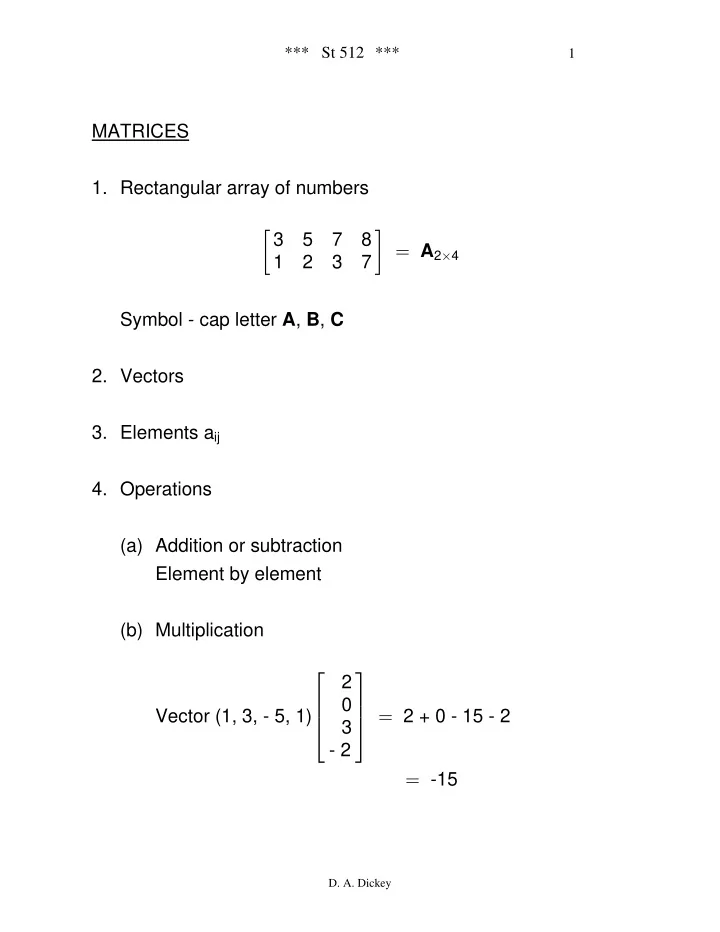
MATRICES

• 1. Rectangular array of numbers

”

• 3

5 7 8 1 2 3 7 œ A2 4

‚

Symbol - cap letter , , A B C

• 2. Vectors
• 3. Elements aij
• 4. Operations

(a) Addition or subtraction Element by element (b) Multiplication Vector (1, 3, - 5, 1) 2 + 0 - 15 - 2 2 3

• 2

Ô × Ö Ù Ö Ù Õ Ø œ

• 15

œ

*** St 512 ***

2

• D. A. Dickey

Matrices ”

• ”
• Ô

× Õ Ø 1 3 5 7 8

• 2
• 1

2

• 2
• 15

2 3 5 1

• 2

œ Note: In general, does not equal BA AB (may have different dimensions) (c) Transpose Aw Note: (AB) (B ) (A )

w w w

œ (d) Scalar Multiplication 3 1 2 3 6

• 2

3

• 6

9 ”

• ”
• œ
• 5. Identity Matrix I

I IA AI A A IB B B CI C C 1 for 1 for 1 for œ œ œ œ œ Ô × Õ Ø

3 3 3 C r 3 ‚ ‚ ‚

*** St 512 ***

3

• D. A. Dickey
• 6. Rank and dependence

A columns , , and 1 1 1 1 1 1 3 1 5 3 1 5 2 3 1 2 3 1 œ œ Ô × Ô × Ô × Ô × Õ Ø Õ Ø Õ Ø Õ Ø Note: 2

• where

is a column of 0's. C C C

1 2 3 œ F

F We say that , , and are linearly . C C C

1 2 3

dependent In general: k columns , , , are dependent there C C C

1 2 k

á if exist scalars , , , such that

• 1

2 k

á (1) + + +

• 1

1 2 2 k k

C C C á œ F and (2) At least one of the 's is 0.

• not

If the k columns are not dependent we call them linearly

• independent. The combination of columns in (1) is called a

linear combination, a phrase we will often use. Thus, k columns are linearly independent if the only linear combination

• f them which will produce the zero vector is the linear

combination with all 's 0. Often we will collect the 's together

• in a vector .

A The

• f a matrix is the maximum number of linearly

rank independent columns which can be selected from the columns

• f the matrix. Thus the rank of is two. Notice that if the rank

A

*** St 512 ***

4

• D. A. Dickey
• f a matrix is 1, then there is one column such that all other

columns are direct multiples. For any matrix , the rank of is the same as the rank of X X X X

w . The

rank of any matrix is always equal to the column row rank.

• 7. Inverse of a matrix.

Symbol: A1 The inverse of an n n matrix is an n n matrix ‚ ‚ A B such that . Such a matrix will exist only if is of rank AB I B A œ

• n. In this case it is also true that

. BA I œ Example: A A 1

• 1

1 0.5 1

• 0.5

2 1

• 1.0
• 1

1.0 3 1 1

• 0.5
• 2

1.5 œ œ Ô × Ô × Õ Ø Õ Ø

1

(Check by multiplication.)

*** St 512 ***

5

• D. A. Dickey

Solving equations b b b 2

1 2

  œ b b 7 2 0

1

 œ b b b

• 5

3 0

1 2

  œ 1

• 1

1 b 2 2 1 b 7 3 1 1 b

• 5

Ô × Ô × Ô × Õ Ø Õ Ø Õ Ø

1 2

œ b 0.5 1

• 0.5

2 10.5 b

• 1.0
• 1

1.0 7

• 14.0

b

• 0.5
• 2

1.5

• 5
• 22.5

Ô × Ô × Ô × Ô × Õ Ø Õ Ø Õ Ø Õ Ø

1 2

œ œ Ab c b A c œ Ê œ

1

For a 2 2 matrix we have the formula: ‚

• nly

a b d

• b

c d

• c

a ”

• ”
• 1

œ

1 ad - bc

Note: if and are square matrices then A B A B

  1 1 œ

( ) BA 1

*** St 512 ***

6

• D. A. Dickey

RANDOM VECTORS We have described a random variable like univariate weight W by writing W N(150, 100) µ We might also measure height in inches H and have H N(68, 16) µ Now the above tells us nothing about how the two variables height and weight . The between H and W covary covariance tells us how weight depends on height. If we know an individual is taller than the mean 68, would we predict that his weight will exceed the mean 150? If so we are claiming a positive covariance between height and weight. Formally, recall that the variance of weights is defined as an , namely expected value variance (W) E (W - 150) . œ š ›

2

The between W and H is defined as covariance cov (W, H) E (W - 150) (H - 68) . œ š › Suppose the covariance is cov(W, H)

• 30. We put this all

œ together as

*** St 512 ***

7

• D. A. Dickey

”

• ”
• ”
• –

— W 150 100 30 H 68 30 16 MVN , µ In general we write Y V MVN ( , ) µ . where is a vector with i element Y , is a vector with i Y

th th i .

element and is a matrix whose ij element is the covariance .i

th

V between Y and Y .

i j

******* ******* Fact: If and are matrices of constants and Y is a A B ******* random vector with ******* MVN ( , ) Y V µ . then + MVN ( + , ) AY B A B AVA µ .

w

Example: Y MVN , 4 8 5 6 5 12 4 10 4 9 µ Ô × Ö Ù Ö Ù Õ Ø Ô × Ô × Õ Ø Õ Ø (1) Find the distribution of Z Y - Y + Y . œ

1 2 3

(2) Let W Y - 3Y + 2Y . Find the joint distribution of Z and œ

1 2 3

W.

*** St 512 ***

8

• D. A. Dickey

REGRESSION - HAND CALCULATION Review of calculations 7 * from first semester: 6 * * 5 * DATA X 4 7 5 4 4 Y 5 7 6 6 3 2 1 2 3 4 5 6 7 X 5, Y 6 – – œ œ

X - X (X - X) Y - Y (Y-Y) (X-X)(Y-Y – – – – – –

2 2

)

• 1

1

• 1

1 1 2 4 1 1 2

• 1

1 === === === === === 6 2 3 slope b 3/6 0.5 œ œ œ intercept a 6 - (0.5)(5) 3.5 œ œ œ True slope . Recall that b N( , /( (X - X) )). – " " 5 D µ

# i 2

True intercept . ! Recall that a N , 1/n + X / (X - X) – – µ   ’ “ ! 5 D

# 2 i 2

*** St 512 ***

9

• D. A. Dickey

Estimate by s (total SSq - regn SSq)/df 5#

# œ

• Regn. SSq

3 * 3/6 1.5 œ œ Total SSq 2 œ df n 2 4 2 2 œ  œ  œ so s MSE (2 1.5)/2 0.25

2 œ

œ  œ Estimated variance of a is 0.25(1/4 25/6) 1.1042  œ Estimated variance of b is 0.25/6 0.041667 œ Notice that 511 formulas gave no indication of . covariance EXAMPLES: Test for no relationship between Y and X. H : =0 , t = = .5 / .041667

b-0

• std. err. of b

" È Give 95% confidence interval for Y at X 6. mean œ 3.5 + .5 (6) = 6.5 = prediction add and subtract t times std. err. of prediction

• std. err. of prediction =

1/n +(6- X) / (X - X) 0.25 – – É ‘

2 2 i

D Give 95% prediction interval for Y at X 6. individual œ same prediction, 6.5

• std. err. of prediction =

1+1/n +(6- X) / (X - X) 0.25 – – É ‘

2 2 i

D

*** St 512 ***

10

• D. A. Dickey

Example of a regression: Wilson and Mather, JAMA 229 (1994) LINE X XSQ XY AGE Y YSQ 9.75 0.552 0.3047 -26.3083 19 -47.66 2271.48 9.00 -0.198 0.0392 5.2787 40 -26.66 710.76 9.75 0.552 0.3047 11.780 21.34 455.40 9.00 -0.198 0.0392 -5.413 27.34 747.48 ====== ======= ======== ======= ======= 0 78.4098 -107.18 0.00 9755.22 Wilson and Mather, JAMA 229 (1994) Plot of AGE*LINE. Legend: A = 1 obs, B = 2 obs, etc. Plot of YHAT*LINE. Symbol used is '-'. ‚ +-----------------------------------+ 100 ˆ | ^ | ‚ | Age = 79.2334 - 1.367 * Line | ‚ A | | ‚ +-----------------------------------+ ‚ A A ‚ A ‚ A A A A 80 ˆ A A ‚ A A g ‚ A A A A A A e ‚ -------- A C A ‚ ----------A-A--------AA A a ‚ A B--B-----A---A------- t ‚ A A --------------------- 60 ˆ A ----- D ‚ AA A A A e ‚-------------------------+ A a ‚ MSE estimates variance | A t ‚ around line. 50 obsns. | A h ‚ | A ‚ MSE is 2 | A A +---------------------------------------+ 40 ˆ (-107.18) | A | b = -107.184 / 78.4094 = -1.367 | ‚ 9755.22 - -------- | | Is b estimating 0 ? | ‚ 78.4098 | | 1. Variance of b is MSE/78.4098 | ‚ ----------------- | | = 200.181 / 78.4098 = 2.553 | ‚ 48 | | 2. Standard error is square root | ‚ | | of 2.553 so it is 1.5978. | ‚ = 200.181 | | 3. t = b/1.5978 = -0.86 | 20 ˆ | A | (not significant) | Šƒƒˆƒƒƒƒƒƒƒƒƒˆƒƒƒƒƒƒƒƒƒˆƒƒƒƒƒƒƒƒƒˆƒƒƒƒƒƒƒƒƒˆƒƒƒƒƒƒƒƒƒˆƒƒƒƒƒƒƒƒƒˆƒƒƒƒƒƒƒƒƒˆƒƒƒƒƒƒƒƒƒˆƒƒ 6 7 8 9 10 11 12 13 14 Length of Lifeline (cm.)

*** St 512 ***

11

• D. A. Dickey

Discussion of correlation coefficients: We define the (population) between two correlation variables as the covariance divided by the square root of the product of the variances. For height and weight as just given, 3 30/ 100*16 0.75. Now suppose we take n 103 œ œ œ È people and measure their height H and weight W . As usual,

i i

we can estimate variances as S (W W) /(n 1) and S (H H) /(n 1). – –

2 2 2 2 W H i i

œ   œ   D D The covariance is estimated as S (W W)(H H)/(n 1). – –

WH i i

œ    D Now these are just estimates of the true values so let us assume we get, say, S 125, S 20, and S 40.

2 2 W H WH

œ œ œ Our estimated covariance matrix is then V 125 40 40 20

^

œ ”

• and we compute a sample estimate, r, of as

3 r 40/ 125*20 0.8. œ œ È

*** St 512 ***

12

• D. A. Dickey

Notice that r regression SS/total SS

2 (W W)(H H) – – (W W) (H H) – –

œ œ

 ‘ D D D

i i 2 i i 2 2

   

from a regression of either H on W or of W on H. Thus we have explained 64% of the variability in W by regressing it on H. A test that 0 is just the t-test on the coefficient in the 3 œ regression of W on H (or equivalently H on W). To test any

• ther hypothesis like H :

0.5 or to put a confidence interval

0 3 œ

around r, Fisher's transformation to Z is used. We define Z 0.5 ln((1 r)/(1 r))

r œ

  and define Z similarly. Now approximately we have

3

Z N(Z , 1/(n 3)).

r µ



3

Thus we get Z 1.09861 so

0.8 œ

1.09861 0.196  and 1.09861 0.196  are the lower and upper confidence bounds for Z .

3

Converting from Z to we get 0.71 0.86. Table A.12

3

3 3 Ÿ Ÿ can be used to do the conversions or simply do them on a hand calculator.

*** St 512 ***

13

• D. A. Dickey

REGRESSION IN MATRIX FRAMEWORK The equations: (Henceforth intercept is , slope is ) " "

1

5 4 e œ   " "

1 1

7 7 e œ   " "

1 2

6 5 e œ   " "

1 3 Y X e ; i 1, 2, 3, 4 Ê œ   œ

i 1 i i

" "

6 4 e œ   " "

1 4

Matrix form: Ô × Ô × Ô × Ö Ù Ö Ù Ö Ù Ö Ù Ö Ù Ö Ù Õ Ø Õ Ø Õ Ø ”

• 5

1 4 e 7 1 7 e 6 1 5 e 6 1 4 e œ  Ê œ  " "

! # " $ " %

Y X e " Estimate by such that ( ) ( ) is minimized. " b Y Xb Y Xb  

w

Note: this is the

• f residuals

. sum of squares Y Xb  Using calculus we can show the sum of squares is minimized by solving the following “normal equations." ******** ******** ( ) i.e. b ( ) ( ) X X b X Y X X X Y

w w w  w

œ œ

1

******** THIS FORMULA IS IMPORTANT

*** St 512 ***

14

• D. A. Dickey

Our little example: X X X X

w w  

( ) 4 20 106 20 20 106 20 4 œ Ê œ   ”

• ”
• 1

1 424 400

We find the solution b 4.4167 0.8333 24 3.5 0.8333 0.1667 123 0.5 œ œ   ”

• ”
• ”
• Now let's relate the vector of

parameters ( ) to the estimated b vector of parameters ( ). We have actual " ( ) ( ) ( ) ( ( )) b X X X Y X X X X e œ œ  œ

w  w w  w 1 1

" ( ) ( ). "  X X X e

w  w 1

The difference between and is ( ) ( ). b b X X X e " "  œ

w  w 1

Results: (1) is an estimate of . b unbiased "

*** St 512 ***

15

• D. A. Dickey

(2) The variance-covariance matrix of ( ) is related to b Vb that of ( ) by the formula e Ve V X X X V X X X

b 1 1 e

(( ) ( ) ) œ

w  w w 

(3) Let us assume that all the e's have the same variance, have mean 0, and are uncorrelated. That means V I

e

œ 5# and after all the smoke clears, we obtain the crucial formula ******** ******** var( ) ( ) V b X X

b 1

œ œ

w  #

5 ******** ESTIMATION OF VARIANCE OF e (1) Sum of squared residuals (sum of squared errors, SSE) vector of residuals Y Xb  For any vector , is sum of squared elements a a a

w

*** St 512 ***

16

• D. A. Dickey

SSE (Y Xb) (Y Xb) œ  

w

Y Y b X Y Uncorr. Total SSq Uncorr.

• Regn. SSq

œ 

w w w

(Y Y ny ) (b X Y ny ) – – Corrected Corrected total SSq

• Regn. SSq

œ   

w w w 2 2

(2) Error df = n - 2 (2 = one intercept + one slope) MSE = SSE/df (3) For our little example, check this against ST511 formula. (4) degrees of freedom will always give degrees of Error freedom for statistics. t Example (Continued.) Variance-covariance matrix of parameter estimates Vb (0.25) 4.4167

• 0.8333

1.1042

• 0.2083
• 0.8333

0.1667

• 0.2083

0.0417 œ œ ”

• ”
• (1) Test that slope is 0: t

0.5 / 0.0417 (2 degrees of freedom) œ È 0.5 / 0.2041 2.45 œ œ

*** St 512 ***

17

• D. A. Dickey

(2) Test that intercept is 0: t 3.5 / 1.1042 3.33 (2 degrees of freedom) œ œ È (3) Estimate mean value of Y at X 6 and give 95% œ confidence interval. Estimate is 3.5 + 0.5 * 6 6.5 œ We are estimating + 6 (1, 6) " " " "

1 œ

”

• !

"

Our estimate is (1, 6) = b + 6b 3.5 + (6)(0.5) 6.5 b

1 œ

œ Letting (1, 6) we now want the variance of but we A A

w w

œ b know how to get that: Var ( ) = (1, 6) = 0.1042 1.1042

• 0.2083

1

• 0.2083

0.0417 6 A A A

w w

b V =

b

”

• ”
• 95% confidence interval : 6.5

t * 0.1042 „ È (4) Predict future individual value at X 6 œ Individual will differ from mean by a deviation with variance estimated by MSE 0.25. Any future individual value at X œ œ 6 is equal to mean at X 6 plus deviation. Thus the variance œ is the sum of the variances of these two parts, namely, 0.25 0.1042 0.3542. Notice that the prediction interval  œ

*** St 512 ***

18

• D. A. Dickey

for an individual future value is wider than the corresponding confidence interval for the mean. We get, for our little example, 6.5 t * 0.3542 „ È Since t has 2 d.f. we obtain t 4.30 and thus œ Confidence interval (5.11, 7.89) Prediction interval (3.94, 9.06) Example: You are in charge of predicting wheat yields from rainfall through July for your country so that you can place import quotas in early August. You have historic data on rain and yields. Which of the above formulas do you use and why? Example: An industrial quality control expert takes 200 hourly measurements on an industrial furnace which is under control and finds that a 95% confidence interval for the mean termperature is (500.35, 531.36). As a result he tells management that the process should be declared out of control whenever hourly measurements fall outside this interval and, of course, is later fired for incompetence. (Why and what should he have done?)

*** St 512 ***

19

• D. A. Dickey

SUMMARY OF REGRESSION FORMULAS Model: where MVN(0, ) Y X e e I œ  µ " 5# Normal Equations: X X b X Y

w w

œ Solution: ( ) ( ) provided is full rank b X X X Y X X œ

w  w w 1

Estimate of variance-covariance matrix of : ( ) MSE b X X

w 1

Predictions for observed Y's is: vector . Xb We write Y Xb (^ denotes predictor). ^ œ Residuals: œ  Y Xb SSE ( ) ( ) œ   œ  œ Y Xb Y Xb Y Y b X Y

w w w w

total SSq

• regn. SSq.

 df n minus rank of matrix. œ X (Usually, rank number of columns in , i.e. rank.) œ X full Prediction of future Y's at some configuration of X's: Prediction written as Y where (1, X-values). In ^ œ œ A A

w w

b

• ur example

(1, 6). Aw œ

*** St 512 ***

20

• D. A. Dickey

Variances of predictions: for mean at configuration of X's in : A ( ( ) ) MSE A A

w w 

X X

1

for individual at configuration of X's in : A ( ( ) 1) MSE A A

w w 

X X

1

 ANOVA (Column of 1's and k other columns.)

SOURCE DF SSq model k

• CT Note: CT= correction term

ny – b X Y

w w

œ

2

error n k 1    Y Y b X Y

w w w

total n 1 Y Y CT  

w

R = coefficient of determination

2

= corrected regn. SSq/corrected total SSq. = 1 SSq(error)/SSq(corrected total)  F = MS(MODEL)/MS(ERROR)

n k 1 k  

tests H : = = = = 0

1 2 k

" " " â

*** St 512 ***

21

• D. A. Dickey

TYPE I (sequential) and TYPE III (partial) SUMS OF SQUARES DATA Y 1 2 X X X 2 1 2 1

• 3

1 1

• 1

2 2 1 1 2 ( ) X X X X X Y b

w w  w 1

REGRESS Y ON X0 ONLY 4 1/4

• 3
• 3/4

(SSR = 9/4 2.25 CT) œ œ œ b X Y

w w

REGRESS Y ON X0, X1 4 1/4

• 3
• 3/4

10 1/10 9 9/10 ”

• ”
• ”
• ”
• (SSR

= 2.25 + 8.1 10.35) œ œ b X Y

w w

REGRESS Y ON X0, X1, X2

Ô × Ô × Ô ×Ô × Õ Ø Õ Ø Õ ØÕ Ø 4 3 10/22

• 3/11
• 3
• 21/11

10 1/10 9 9/10 3 5

• 3/11

4/11 2 17/11

(SSR 16.92) œ

*** St 512 ***

22

• D. A. Dickey

Notes: No change in b0 from 1 to 2 regression

st nd

(orthogonality). Two b's change from 2 to 3 (not orthogonal).

nd rd

Adding X2 to regression 2 increases the regression sum of squares from 10.35 to 16.92. We write R(X0, X1, X2) 16.92 œ R(X0, X1) 10.35 œ R(X2 | X0, X1) 6.57 R(X0, X1, X2) R(X0, X1) œ œ  TYPE I SSq TYPE III SSq (sequential) (partial) SOURCE X1 R(X1 | X0) 8.1 R(X1 | X0, X2) 8.1 œ œ (NOT usually equal) X2 R(X2 | X0, X1) 6.57 œ R(X2 | X0, X1) 6.57 œ (always equal) Note: The only reason type I and type III are equal for X1 is

• rthogonality

not . Generally they are

• equal. Obviously type I

œ type III for the last X you have (X2 in our case). Note: Partial SSq is "Type II" in PROC REG, " Type III " in GLM.

*** St 512 ***

23

• D. A. Dickey

EXAMPLE 2: DATA Y 1 X2 X X 2 1 2 1

• 3

1 1

• 1

2 2 1 1 3 Y Y 17 SS(total) 17 - 9/4 14.75

w

œ œ œ ( ) X X X X X Y b

w w  w 1

REGRESS Y ON X0 ONLY 4 1/4 - 3 - 3/4 ( SSR = 9/4 2.25 CT) œ œ œ b X Y

w w

( SSR is "uncorrected") REGRESS Y ON X0, X1

”

• ”
• ”
• ”
• 4

2 10/36

• 2/36
• 3
• 1.0

2 10

• 2/36

4/36 3 0.5

(SSR = 3 + 1.5 4.5) œ œ b X Y

w w

R(X1 | X0) 4.5 - 2.25 2.25 œ œ

*** St 512 ***

24

• D. A. Dickey

REGRESS Y ON X0, X1, X2 ( ) X X X X X Y b

w w  w 1

Ô ×Ô ×Ô ×Ô × Õ ØÕ ØÕ ØÕ Ø 4 2 4 0.4670

• 0.0755
• 0.1792
• 3
• 2.3443

2 10 1

• 0.0755

0.1132 0.0189 3 0.6415 4 1 10

• 0.1792

0.0189 0.1698 4 1.2736

(SSR =14.052) œ b X Y

w w

R(X0, X1, X2) 14.052 œ R(X0, X1) 4.500 œ R(X2 | X0, X1) 9.552 R(X0, X1, X2) R(X0, X1) œ œ  TYPE I SSq TYPE III SSq (sequential) (partial) SOURCE X1 R(X1 | X0) 2.25 œ R(X1 | X0, X2) ______ œ X2 R(X2 | X0, X1) 9.552 œ R(X2 | X0, X1) 9.552 œ EXERCISE: Fill in the blank above by regressing Y on X0 and X2, etc. Are type I and type III equal for X1 in this example?

(ANS: 3.6353, .) no

*** St 512 ***

25

• D. A. Dickey

GRADE – IQ EXAMPLE IQ TIME RADE STUDY G 105 75 1 110 2 79 1 120 6 68 116 3 85 1 122 6 91 1 130 8 79 114 98 2 102 5 76 1 Use the class computing account to enter the study time data. Regress GRADE on IQ. Regress GRADE on TIME, IQ. Finally, regress GRADE on TIME IQ TI where TI TIME*IQ. The TI œ variable could, for example, be created in your data step. For the regression of GRADE on TIME and IQ, use the option /I in PROC REG. This will output the ( ) matrix. X X

w 1

ANOVA (Grade on IQ) Source df SSq Mn Sq F IQ 1 15.9393 15.9393 0.153 Error 6 25.935 104.32 6

*** St 512 ***

26

• D. A. Dickey

It appears that IQ has nothing to do with grade, but we did not look at study time. Looking at the multiple regression we get ANOVA (Grade on IQ, Study Time) Source df SSq Mn Sq F Model 2 96.12 98.06 2.57 5 2 3 Error 5 45.76 9.15

TYPE I TYPE III (sequential) (partial)

SOURCE df IQ 1 15.94 21.24 1 STUDY 1 80.18 80.18 5 5

Parameter Estimate t Pr > |t|

• Std. Err.

INTERCEPT 0.74 0.05 0.9656 16.26

0.9851

IQ 0.47 3.64 0.0149 0.13 ___|__________|__ STUDY 2.10 7.96 0.0005 0.26 3.64 3.64 

From this regression we also can get ( ) .8985 .2261

• .2242

28

• .2261

.0018 .0011

• .2242

.0011 .0076

• X X

w

• 1 œ

Ô × Õ Ø

• 1. To test H0: Coefficient on IQ is 0 (Note: calculations done

with extra decimal accuracy.) (a) Using t-test t 0.47/ 0.0018*9.15 3.64 œ œ È (b) Using type III F-test, F 121.24/9.15 13.25 t . œ œ œ

2

*** St 512 ***

27

• D. A. Dickey

Note: The type III sum of squares is defined by setting t F.

2 œ

This means that type III SSq b*b/c where b is the coefficient œ being tested and c is the diagonal element of ( ) which X X

w 1

corresponds to b. We have (0.47)(0.47)/0.0018 121.24. œ

• 2. Estimate the mean grade for the population of all potential

students with IQ 113 and study time 14 hours. œ œ (a) Write this estimate as where (1, 113, 14). A A

w w

b œ (b) Variance of this is ( ) *MSE 1.303. A A

w w 

X X

1

œ (c) Prediction is 83.64. Awb œ (d) To get confidence interval, 83.64 2.571 1.303 „ È (e) Interval (80.71, 86.57)

• 3. Estimate grade for

with 113 IQ and 14 hours study individual time. 83.64 2.571 1.303 9.15 „  È (75.33, 91.95)

• 4. What percent of grade variability is explained by IQ,

STUDY?

*** St 512 ***

28

• D. A. Dickey

R = (corrected regn. SSQ)/(corrected total SSq)

2

œ 596.12/641.88 93% œ

• 5. Notes: When a new column is added to a regression,

the all coefficients and their t-statistics can change. The t's could go from significance to insignificance vice-versa.

• r

The exception to the above case is when the added column of is to the original columns. This means X

• rthogonal

that the new has the old in the upper left corner, the X X X X

w w

sum of squares of the new column as the bottom right element, and all other elements 0. Rerun this example adding a row 113 14 . at the end of the

• dataset. The dot implies a missing value. Use the statement

MODEL GRADE IQ STUDY / P CLM; . Compare to part 2 œ

• above. Rerun again with CLI instead of CLM. Compare to part

3 above. Was the extra data row used in computing the regression coefficients?

OPTIONS LS 80 NODATE; œ DATA GRADES; INPUT IQ STUDY GRADE @@; ST_IQ STUDY*IQ; CARDS; œ 105 10 75 110 12 79 120 6 68 116 13 85 122 16 91 130 8 79 114 20 98 102 15 76 PROC REG; MODEL GRADE IQ STUDY ST_IQ/SS1 SS2; œ TITLE “GRADE AND STUDY TIME EXAMPLE FROM ST 512 NOTES"; PROC PLOT;

*** St 512 ***

29

• D. A. Dickey

PLOT STUDY*IQ * / VPOS 35; œ œ

w w

DATA EXTRA; INPUT IQ STUDY GRADE; CARDS; 113 14 . DATA BOTH; SET GRADES EXTRA; PROC REG; MODEL GRADE IQ STUDY/P CLM; œ RUN;

GRADE AND STUDY TIME EXAMPLE FROM ST512 NOTES DEP VARIABLE: GRADE

SUM OF MEAN SOURCE DF SQUARES SQUARE F VALUE PROB>F MODEL 3 3 7 3 610.81 203.60 26.21 0.004 ERROR 4 4 9 31.06467 7.76616 C TOTAL 7 5 641.87 ROOT MSE 5 E 6 2.78678 R-SQUAR 0.951 DEP MEAN Q 3 81.37500 ADJ R-S 0.915 C.V. 2 3.4246

R D : PARAMETE STANDAR T For H0 VARIABLE DF E R | S ESTIMAT ERRO PARAMETER PROB>|T TYPE I S œ

INTERCEP 1 6 6 5 7 5 72.20607 54.07277 1.33 0.252 52975.12 IQ 1 8 6 9 0.13117 0.45530 0.28 0.787 15.93929   STUDY 1 2 1 9 9 6 4.11107 4.52430 0.90 0.414 580.17   ST IQ 1 1 1 6 0.05307 0.03858 1.37 0.241 14.69521 _ VARIABLE DF S TYPE II S INTERCEP 1 6 13.84831 IQ 1 9 0.64458 STUDY 1 3 6.41230 ST IQ 1 14.69521 _

*** St 512 ***

30

• D. A. Dickey

Discussion of the interaction model. We call the product I * S IQ * STUDY an “interaction" term. Our model is œ G 72.21 0.13 I 4.11 S 0.0531 I * S. ^ œ    Now if IQ 100 we get œ G (72.21 13.1) ( 4.11 5.31) S ^ œ     and if IQ 120 we get œ G (72.21 15.7) ( 4.11 6.37) S. ^ œ     Thus we expect an extra hour of study to increase the grade by 1.20 points for someone with IQ 100 and by 2.26 œ points for someone with IQ 120 if we use this interaction œ

• model. Since the interaction is not significant, we may want to

go back to the simpler “main effects" model. Suppose we measure IQ in deviations from 100 and STUDY in deviations from 8. What happens to the coefficients and t-tests in the interaction model? How about the main effects model?

*** St 512 ***

31

• D. A. Dickey

GRADE AND STUDY TIME EXAMPLE FROM CLASS NOTES GRADE AND STUDY TIME EXAMPLE FROM CLASS NOTES Plot of STUDY*IQ. Symbol used is 'X'. Plot of STUDY*IQ. Symbol used is 'X'. STUDY ‚ STUDY ‚ ‚ ‚ ‚ ‚ ‚ ‚ 20 ˆ X 20 ˆ X 19 ˆ 19 ˆ 18 ˆ 18 ˆ 17 ˆ 17 ˆ 16 ˆ X 16 ˆ X 15 ˆ X 15 ˆ X 14 ˆ 14 ˆ 13 ˆ X 13 ˆ X 12 ˆ X 12 ˆ X 11 ˆ 11 ˆ 10 ˆ X 10 ˆ X 9 ˆ 9 ˆ 8 ˆ X 8 ˆ X 7 ˆ 7 ˆ 6 ˆ X 6 ˆ X ‚ ‚ Šƒˆƒƒƒƒƒƒƒƒƒƒƒƒƒƒˆƒƒƒƒƒƒƒƒƒƒƒƒƒƒˆƒƒƒƒƒƒƒƒƒƒƒƒƒƒˆ Šƒˆƒƒƒƒƒƒƒƒƒƒƒƒƒƒˆƒƒƒƒƒƒƒƒƒƒƒƒƒƒˆƒƒƒƒƒƒƒƒƒƒƒƒƒƒˆ 100 110 120 130 100 110 120 130

*** St 512 ***

32

• D. A. Dickey

GRADE AND STUDY TIME EXAMPLE FROM NOTES DEP VARIABLE: GRADE

SUM OF MEAN SOURCE DF SQUARES SQUARE F VALUE PROB>F MODEL 2 5 8 8 4 596.11 298.05 32.56 0.001 ERROR 5 5 7 45.75988 9.15197 C TOTAL 7 5 641.87 ROOT MSE 3 E 7 3.02522 R-SQUAR 0.928 DEP MEAN Q 2 81.37500 ADJ R-S 0.900 C.V. 3 3.71763

R D : PARAMETE STANDAR T FOR H0 VARIABLE DF E R | ESTIMAT ERRO PARAMETER PROB>|T œ

INTERCEP 1 5 5 6 0.73655 16.26280 0.04 0.965 IQ 1 4 9 0.47308 0.12998 3.64 0.014 STUDY 1 6 4 2 5 2.10343 0.26418 7.96 0.000 T R % % PREDIC STD ER LOWER 95 UPPER 95 OBS TUAL E T N N L AC VALU PREDIC MEA MEA RESIDUA 1 .000 5 3 7 2 5 75 71.44 1.93 66.47 76.41 3.55 2 .000 7 2 2 1 79 78.01 1.27 74.75 81.28 0.98300 3 .000 7 3 2 3 7 68 70.12 1.96 65.08 75.17 2.12  4 .000 9 3 8 1 85 82.95 1.09 80.15 85.76 2.04 5 .000 8 5 6 8 91 92.10 1.83 87.39 96.82 1.10  6 .000 5 2 3 7 8 79 79.06 2.24 73.30 84.82 .06492  7 .000 7 4 9 5 3 98 96.73 2.22 91.01 102.45 1.26 8 .000 3 9 5 3 76 80.54 1.92 75.58 85.50 4.54  9 . 3 1 9 7 . 83.64 1.14 80.70 86.57 SUM OF RESIDUALS 5 7.10543E–1 SUM OF SQUARED RESIDUALS 45.75988

*** St 512 ***

33

• D. A. Dickey

ANALYSIS OF VARIANCE AS A SPECIAL CASE OF REGRESSION First, let us review ANOVA from last semester. Suppose we record the weights of 20 plants, where each of 4 fertilizers is used on one group of 5. We get these yields: DATA (YIELD) MEAN SUM SSq FERTILIZER A 60 61 59 60 60 60 300 2 FERTILIZER B 62 61 60 62 60 61 305 4 FERTILIZER C 63 61 61 64 66 63 315 18 FERTILIZER D 62 61 63 60 64 62 310 10 1230 34 You should remember how to compute this table: ANOVA Source df SSq Mn Sq F FERTILIZER 3 25 8.333 3.92 ERROR 16 34 2.125 TOTAL 19 59

*** St 512 ***

34

• D. A. Dickey

You may also remember how to compare treatment means. CONTRAST I comparing A to B Estimated difference 60 - 61 = - 1 Variance (2.125)(1/5 + 1/5) = 0.85 t-statistic = - 1 / 0.85 = - 1.0847 È CONTRAST II comparing mean of A and B to C (or A + B compared to 2C) Estimate of [A mean + B mean - 2(C mean) = 60 + 61 - 2(63) = - 5 Variance (2.125)(1/5 + 1/5 + 4/5) = 2.55 t-statistic = - 5/ 2.55 = -3.1311 È Finally you may remember the model Y = + + e .

ij i ij

. ! The model says that each yield is an overall mean ( ) plus a . fertilizer effect ( ) plus a random deviation, e . Now we can !i

ij

write this model as a matrix regression using these matrices:

*** St 512 ***

35

• D. A. Dickey

TABLE 1: Y X e " Î Ñ Î Ð Ó Ð Ð Ó Ð Ð Ó Ð Ð Ó Ð Ð Ó Ð Ð Ó Ð Ð Ó Ð Ð Ó Ð Ð Ó Ð Ð Ó Ð Ð Ó Ð Ó Ð Ó Ð Ó Ð Ó Ð Ó Ð Ó Ð Ó Ð Ó Ð Ó Ð Ó Ð Ó Ð Ó Ð Ó Ð Ó Ð Ó Ð Ó Ð Ó Ð Ó Ð Ó Ð Ó Ð Ó Ð Ó Ï Ò 60 61 59 60 60 62 61 60 62 60 63 61 61 64 66 62 61 63 60 64 = Ð Ó Ð Ó Ð Ó Ð Ó Ð Ó Ð Ó Ð Ó Ð Ó Ð Ó Ð Ó Ð Ó Ð Ó Ð Ó Ð Ó Ð Ó Ð Ó Ð Ó Ð Ó Ð Ó Ð Ó Ð Ó Ð Ó Ð Ó Ï Ò Ñ Ó Ó Ó Ó Ó Ó Ó Ó Ó Ó 1 1 1 1 1 1 1 1 1 1 1 1 1 1 1 1 1 1 1 1 1 1 1 1 1 1 1 1 1 1 1 1 1 1 1 1 1 1 1 1 + Î Ñ Ð Ó Ð Ó Ð Ó Ð Ó Ï Ò Î Ñ Ð Ó Ð Ó Ð Ó Ð Ó Ð Ó Ð Ó Ð Ó Ð Ó Ð Ó Ð Ó Ð Ó Ð Ó Ð Ó Ð Ó Ð Ó Ð Ó Ð Ó Ð Ó Ð Ó Ð Ó Ð Ó Ð Ó Ð Ó Ð Ó Ð Ó Ð Ó Ð Ó Ð Ó Ð Ó Ð Ð Ð Ð Ï . ! ! ! !

1 2 3 4

Ó Ó Ó Ó Ò e e e e e e e e e e e e e e e e e e e e

11 12 13 14 15 21 22 23 24 25 31 32 33 34 35 41 42 43 44 45

It is obvious by multiplying the matrix by the vector that X " every observation in the first group is (1) + (1) + (0) + . ! !

1 2

(0) + (0) = + plus an error e, every element in group 2 ! ! . !

3 4 1

is + plus an error, etc. This is the ANOVA model. . !2 exactly Now we are tempted to run a regression of on the columns of Y

*** St 512 ***

36

• D. A. Dickey

X X to get our ANOVA but there is a problem. Look at the

• matrix. Is it full rank? Obviously the answer is no. (Try

inverting in SAS and see what happens.) I will now write X X

w

down a new matrix and vector. X " TABLE 2: Betas X " Ð Ñ 1 1 0 0 is now . ! " 

4 !

1 1 0 0 is now ! ! "

1 4



"

1 1 0 0 is now ! ! "

2 4



#

1 1 0 0 is now ! ! "

3 4



$

1 1 0 0 1 0 1 0 Note: For rows 1 - 5 of , multiplying row of X X 1 0 1 0 times the vector (recall multiplication of row " 1 0 1 0 times column 1 0 1 0 (1)( + ) + (1)(

• ) + 0 + 0 = +

. . ! ! ! . !

4 1 4 1

1 0 1 0 1 0 0 1 1 0 0 1 1 0 0 1 1 0 0 1 1 0 0 1 1 0 0 0 Note: The last 5 rows multiplied by give + " . !4 1 0 0 0 as they should. 1 0 0 0 1 0 0 0 1 0 0 0

*** St 512 ***

37

• D. A. Dickey

For the above matrix and our fertilizer data, put the Y's X and the last three columns of the last matrix in a SAS data X

• set. Call the columns X1, X2, and X3. Regress Y on X1, X2, X3

and notice that you have produced the ANOVA table and F test for treatments (PROC REG supplies the column of 1s). Recall CONTRAST I and CONTRAST II on the previous

• page. We can even make the computer estimate those

contrasts and give us the t-statistics. Here are the matrix X columns to do the job:

*** St 512 ***

38

• D. A. Dickey

TABLE 3: = 1 1 1 1 1 1 1 1 1 1 1 1 1 1 1 1 1 1 1 1 1

• 1

1 1 1

• 1

1 1 1

• 1

1 1 1

• 1

1 1 1

• 1

1 1 1

• 2

1 1 X Î Ñ Ð Ó Ð Ó Ð Ó Ð Ó Ð Ó Ð Ó Ð Ó Ð Ó Ð Ó Ð Ó Ð Ó Ð Ó Ð Ó Ð Ó Ð Ó Ð Ó Ð Ó Ð Ó Ð Ó Ð Ó Ð Ó Ð Ó Ð Ó Ð Ó Ð Ó Ð Ó Ð Ó Ð Ó Ð Ó Ð Ó Ð Ó Ð Ó Ð Ó Ï Ò

• 2

1 60 1

• 2

1 1

• 2

1 1

• 2

1 1

• 3

1

• 3

1

• 3

1

• 3

1

• 3

20 10 30 X X

w

œ Ô × Ö Ù Ö Ù Õ Ø Consider the second element of . It will be X Y

w

(treatment 1 sum) - (treatment 2 sum) = 300 - 305 = Q

*** St 512 ***

39

• D. A. Dickey

Since is the second b estimated will be b1 = X X

w

diagonal (300 - 305)/10 which is simply 1/2 of CONTRAST I. Similarly b2 is some multiple of CONTRAST II and finally b3 will be some multiple of the contrast comparing the mean of A, B, and C to D. The t-statistics will be those computed above for the exactly

• contrasts. Notice that we have used three

contrasts,

• rthogonal

that is, contrasts which give columns in so that is a X X X

w

diagonal matrix. We could easily compute the regression coefficients and their variances by hand since is so nice (or X X

w

just run it on the computer). You can easily compute the following: X Y b

w =

= = 1230 b 1230/20

• 5

b

• 5/10
• 25

b

• 25/30
• 10

b

• 10/60

MSE = 34/16 = 2.125 Ô × Ô × Ô × Ö Ù Ö Ù Ö Ù Ö Ù Ö Ù Ö Ù Õ Ø Õ Ø Õ Ø

1 2 3

SS(regression) = = b X Y

w w

(1230) /20 + (-5) /10 + (-25) /30 + (-10) /60

2 2 2 2

= 75645 + 2.5 + 20.8333 + 1.6667 = 75645 + 25 = CT + 25

*** St 512 ***

40

• D. A. Dickey

From PROC REG or PROC GLM (or easily by hand) you will get: ANOVA SOURCE DF TYPE I SS TYPE III SS X1 1 2.5000 2.5000 X2 1 20.8333 20.8333 X3 1 1.6667 1.6667 ERROR 16 34.0000 COEFFICIENT T-STAT

• STD. ERR.

X1

• .5000
• 1.0847

.4610 = (2.125/10) È X2

• .8333
• 3.1311

.2661 = (2.125/30) È X3

• .1667
• 0.8856

.1882 = (2.125/60) È SUMMARY:

• 1. An ANOVA is just a special case of regression with dummy
• variables. You have several choices as to how to enter the

dummy variables.

• 2. PROC GLM will automatically create k

1 columns from a  single column of k numbers if we use a class statement. For example if we had a column FERT in our dataset with each entry 1, 2, 3, or 4 we could call PROC GLM; CLASS FERT; MODEL YIELD FERT; then the procedure will automatically œ create the columns of table 2 a couple of pages back. It will

*** St 512 ***

41

• D. A. Dickey

lump all the 1 degree of freedom sums of squares into the usual 3 df ANOVA sum of squares (25).

• 3. Because we had

contrasts (X X diagonal) the

• rthogonal

w

hand computations were easy the TYPE I and TYPE III and sums of squares were exactly the same. Also note that you could have produced exactly the same coefficients and regression sums of squares by running simple linear regressions on each individual column of X. This computational simplicity is due solely to orthogonality.

• 4. You could also throw in 4 columns of

indicator block variables if the experiment had been blocked. Example with treatments in blocks % $ Y int blk blk trt trt trt

ij

") " " ! " ! ! ## " " ! ! " ! $# " " ! ! ! " $$ " " ! ! ! ! #& " ! " " ! ! #( " ! " ! " ! $! " ! " ! ! " $& " ! " ! ! ! "# " ! ! " ! ! "% " ! ! ! " ! #! " ! ! ! ! " #% " ! ! ! ! ! (Of course these could be replaced with columns of CONTRASTS as well).

*** St 512 ***

42

• D. A. Dickey

SAS code for FERTILIZER example: DATA FERT; INPUT FERT $ YIELD @@; X1=(FERT='A'); X2=(FERT='B'); X3=(FERT='C'); X4=(FERT='D'); CARDS; A 60 A 61 A 59 A 60 A 60 B 62 B 61 B 60 B 62 B 60 C 63 C 61 C 61 C 64 C 66 D 62 D 61 D 63 D 60 D 64 ; PROC PRINT; TITLE "FERTILIZER DATA SET"; PROC GLM; CLASS FERT; MODEL YIELD=FERT/SOLUTION; TITLE "CLASS STATEMENT IN GLM"; PROC REG; MODEL YIELD=X1 X2 X3; TITLE "CREATING YOUR OWN DUMMY VARIABLES"; RUN;

*** St 512 ***

43

• D. A. Dickey

FERTILIZER DATA SET FERTILIZER DATA SET OBS FERT YIELD X1 X2 X3 X4 OBS FERT YIELD X1 X2 X3 X4 1 A 60 1 0 0 0 1 A 60 1 0 0 0 2 A 61 1 0 0 0 2 A 61 1 0 0 0 3 A 59 1 0 0 0 3 A 59 1 0 0 0 4 A 60 1 0 0 0 4 A 60 1 0 0 0 5 A 60 1 0 0 0 5 A 60 1 0 0 0 6 B 62 0 1 0 0 6 B 62 0 1 0 0 7 B 61 0 1 0 0 7 B 61 0 1 0 0 8 B 60 0 1 0 0 8 B 60 0 1 0 0 9 B 62 0 1 0 0 9 B 62 0 1 0 0 10 B 60 0 1 0 0 10 B 60 0 1 0 0 11 C 63 0 0 1 0 11 C 63 0 0 1 0 12 C 61 0 0 1 0 12 C 61 0 0 1 0 13 C 61 0 0 1 0 13 C 61 0 0 1 0 14 C 64 0 0 1 0 14 C 64 0 0 1 0 15 C 66 0 0 1 0 15 C 66 0 0 1 0 16 D 62 0 0 0 1 16 D 62 0 0 0 1 17 D 61 0 0 0 1 17 D 61 0 0 0 1 18 D 63 0 0 0 1 18 D 63 0 0 0 1 19 D 60 0 0 0 1 19 D 60 0 0 0 1 20 D 64 0 0 0 1 20 D 64 0 0 0 1 CLASS STATEMENT IN GLM CLASS STATEMENT IN GLM General Linear Models Procedure General Linear Models Procedure Class Level Information Class Level Information Class Levels Values Class Levels Values FERT 4 A B C D FERT 4 A B C D Number of observations in data set = 20 Number of observations in data set = 20

*** St 512 ***

44

• D. A. Dickey

Dependent Variable: YIELD Dependent Variable: YIELD Sum of Mean Sum of Mean Source DF Squares Square F Value Pr > F Source DF Squares Square F Value Pr > F Model 3 25.000000 8.333333 3.92 0.0283 Model 3 25.000000 8.333333 3.92 0.0283 Error 16 34.000000 2.125000 Error 16 34.000000 2.125000 Corrected Total 19 59.000000 Corrected Total 19 59.000000 R-Square C.V. Root MSE YIELD Mean R-Square C.V. Root MSE YIELD Mean 0.423729 2.370306 1.4577 61.500 0.423729 2.370306 1.4577 61.500 Source DF Type I SS Mean Square F Value Pr > F Source DF Type I SS Mean Square F Value Pr > F FERT 3 25.000000 8.333333 3.92 0.0283 FERT 3 25.000000 8.333333 3.92 0.0283 Source DF Type III SS Mean Square F Value Pr > F Source DF Type III SS Mean Square F Value Pr > F FERT 3 25.000000 8.333333 3.92 0.0283 FERT 3 25.000000 8.333333 3.92 0.0283 T for H0: Pr > |T| Std Error of T for H0: Pr > |T| Std Error of Parameter Estimate Parameter=0 Estimate Parameter Estimate Parameter=0 Estimate INTERCEPT 62.0000 B 95.10 0.0001 0.65192024 INTERCEPT 62.0000 B 95.10 0.0001 0.65192024 FERT A -2.0000 B -2.17 0.0455 0.92195445 FERT A -2.0000 B -2.17 0.0455 0.92195445 B -1.0000 B -1.08 0.2941 0.92195445 B -1.0000 B -1.08 0.2941 0.92195445 C 1.0000 B 1.08 0.2941 0.92195445 C 1.0000 B 1.08 0.2941 0.92195445 D 0.0000 B . . . D 0.0000 B . . . NOTE: The X'X matrix has been found to be singular and a NOTE: The X'X matrix has been found to be singular and a generalized inverse was used to solve the normal equations. generalized inverse was used to solve the normal equations. Estimates followed by the letter 'B' are biased, and are not Estimates followed by the letter 'B' are biased, and are not unique estimators of the parameters. unique estimators of the parameters.

*** St 512 ***

45

• D. A. Dickey

CREATING YOUR OWN DUMMY VARIABLES CREATING YOUR OWN DUMMY VARIABLES Model: MODEL1 Model: MODEL1 Dependent Variable: YIELD Dependent Variable: YIELD Analysis of Variance Analysis of Variance Sum of Mean Sum of Mean Source DF Squares Square F Value Prob>F Source DF Squares Square F Value Prob>F Model 3 25.00000 8.33333 3.922 0.0283 Model 3 25.00000 8.33333 3.922 0.0283 Error 16 34.00000 2.12500 Error 16 34.00000 2.12500 C Total 19 59.00000 C Total 19 59.00000 Root MSE 1.45774 R-square 0.4237 Root MSE 1.45774 R-square 0.4237 Dep Mean 61.50000 Adj R-sq 0.3157 Dep Mean 61.50000 Adj R-sq 0.3157 C.V. 2.37031 C.V. 2.37031 Parameter Estimates Parameter Estimates Parameter Standard T for H0: Parameter Standard T for H0: Variable DF Estimate Error Parameter=0 Prob > |T| Variable DF Estimate Error Parameter=0 Prob > |T| INTERCEP 1 62.0000 0.65192024 95.104 0.0001 INTERCEP 1 62.0000 0.65192024 95.104 0.0001 X1 1 -2.0000 0.92195445 -2.169 0.0455 X1 1 -2.0000 0.92195445 -2.169 0.0455 X2 1 -1.0000 0.92195445 -1.085 0.2941 X2 1 -1.0000 0.92195445 -1.085 0.2941 X3 1 1.0000 0.92195445 1.085 0.2941 X3 1 1.0000 0.92195445 1.085 0.2941

*** St 512 ***

46

• D. A. Dickey

5 ˆ | | 3 2 ‚ | 2 | Y= .85 X - 5 X + 7 X + 1 ‚ | Y = X - 4x + 4 | 4 ˆ Y = 1 + .5X | A | BA ‚ | A A | B BA ‚ | A A | A A A 3 ˆ ABA | A A | A AA ‚ ABBAA | A A | A A A ‚ AABB | A A | A A 2 ˆ ABABA | A A | A A ‚ ABBAA | A A | A AA A ‚ AABB | B B | A 1 ˆ ABA | A A | A A A ‚ | B B | AA A ‚ | BA AB | B B 0 ˆ----------------------------+------------BBABB------------+------------------ A-A -------- 3 2 4 3 2 4 3 2 ‚ Y = .17 X -.8 X Y = .5 X -4 X + 10.2 X Y= .25 X - 2 X + 6 X 4 ˆ + 1.4 X + .2 A | -8.8 X + 2.8 | A -8X + 4 ‚ A | | ‚ A | | A A 3 ˆ A | | ‚ AA | A A | A A ‚ B | | 2 ˆ B | A ABABA A | A A ‚ BA | AA AA | A A ‚ BBAB | A B B A | A A 1 ˆ ABABBABBA | A B B A | A A ‚ BAA | A AA AA A | AA AA ‚ AB | ABA ABA | AA AA 0 ˆ----------------------------+-----------------------------+---------BBABBABBABB------------ 2 Y = -X + 3X + 1 2 Y = -.25 X + 4 4 ˆ | ABBABA ‚ | AABB ‚ BAB | ABA 3 ˆ AAB BAA | AAA ‚ AA AA | AB ‚ AA AA | AB 2 ˆ A A | B ‚ AA AA | AA ‚ A A | AA 1 ˆ A A | AA ‚ A | B ‚ A | B 0 ˆ A | ‚ | Šƒˆƒƒƒƒƒˆƒƒƒƒƒˆƒƒƒƒƒˆƒƒƒƒƒˆƒƒ+ƒƒˆƒƒƒƒƒˆƒƒƒƒƒˆƒƒƒƒƒˆƒƒƒƒƒˆƒƒƒƒƒˆƒƒƒƒƒˆƒƒƒƒƒˆƒƒƒƒƒˆƒƒƒƒƒˆƒƒ 0 1 2 3 4 0 1 2 3 4 0 1 2 3 4

*** St 512 ***

47

• D. A. Dickey

POLYNOMIAL REGRESSION Polynomial means form Y + X + X + + X œ â " " " "

1 2 k k #

EXAMPLE: We try work crews of various sizes and record the number of parts produced in an hour for each work crew. We see that up to a point, increasing the number of workers increases per worker production but beyond that point, production begins to decrease. Our goal is to model per worker production as a function of crew size. DATA ( )

Y=PARTS PER WORKER, X=CREW SIZE

Y 3 5 7 12 8 10 10 5 6 4 mean 7 œ X 2 2 3 4 4 4 5 5 5 6 mean 4 œ Mean SSq df 2 3, 5 4 2 1 3 7 7 4 12, 8, 10 10 8 2 5 10, 5, 6 7 14 2 6 4 4 sum = 24 ANOVA Source df SSq Mn Sq F Pr>F Size 4 54 13.5 2.81 0.1436 Error 5 24 4.8

*** St 512 ***

48

• D. A. Dickey

Note: The ANOVA essentially fits means to each crew size. Below we plot the production against crew size and indicate the fitted means from the ANOVA model. Note the ANOVA error sum of squares, 24, is just the pooled (summed) SSq from within each treatment group. The predictions (group means) are not constrained in any way. Data plot: PARTS 12 X 11 10

• X- X

Line segments are ANOVA 9 treatment means. 8 X 7

• X-
• 6

X 5 X X 4

• X-

3 X 2 ---------

• +-----+-----+-----+-----+------------

CREW SIZE — 2 3 4 5 6 Next we will fit a quadratic to the data (forcing predicted values to lie on a parabola) and observe how much the fit deteriorates.

*** St 512 ***

49

• D. A. Dickey

DATA A; INPUT Y X XSQ; CARDS; 3 2 4 5 2 4 7 3 9 4 6 1 1 8 4 6 1 2 4 6 1 1 5 5 5 2 5 5 1 2 6 5 5 2 4 6 6 3 PROC REG; MODEL Y X XSQ; œ The output contains the following information: SOURCE DF SSq Mn Sq F Pr>F MODEL 2 49.42 24.71 6.05 0.0298 ERROR 7 28.58 4.08 PARAMETER ESTIMATE T PR>| T | INTERCEPT

• 12.5280
• 2.19

.0644 X 11.0311 3.47 .0104 XSQ

• 1.3975
• 3.40

.0115 The job can be done more easily in PROC GLM. In fact, we will do several steps: (1) Do an ANOVA of production with crew size as treatment. (2) Fit a quadratic to the data. (3) Fit a degree 4 polynomial to the data. (For only 5 distinct X values, a degree 4 polynomial is the highest degree you can fit.)

*** St 512 ***

50

• D. A. Dickey

PROC GLM; CLASS X; MODEL Y X; œ Try this and you will get a printout like this: (this is the computerized way of getting the ANOVA table). GENERAL LINEAR MODELS PROCEDURE CLASS LEVEL INFORMATION CLASS LEVELS VALUES CREW 5 2 3 4 5 6 SOURCE DF SSq Mn Sq F MODEL 4 54 13.5 2.81 ERROR 5 24 4.8 SOURCE DF TYPE I SS TYPE III SS X 4 54 54 Notice that SAS has created an matrix like table 2 a few X pages back, because we used a CLASS statement. Also, it will not give individual coefficients etc. because of the lack of a unique parameterization (they can be recovered through the /SOLUTION option.) Notice also that the ANOVA, which basically fits group means to the 5 treatment groups, has increased the regression sum of squares over that of the quadratic, from 49.4161 (2df) to 54 (4df). Later, we will show that the ANOVA (means) model is like a “full model" and the quadratic like a “reduced model." The test which asks if the regression does as well as the ANOVA in fitting the data is called a “lack of fit F test." We compute

*** St 512 ***

51

• D. A. Dickey

F (54 49.4161)/2 / (4.8) 0.4775 œ  œ c d Since F is insignificant (2 and 5 df) we say there is no significant lack of fit. We conclude that a model forcing production to be a quadratic in crew size seems to explain production as well as a model in which unconstrained means are fit to the data. To show that the F test is a full versus reduced model F test, I will show that the ANOVA approach is the same as fitting the highest degree polynomial possible to the data. Since there are m = 5 values of X, the highest possible degree is m - 1 = 4. Thus we issue the commands: PROC GLM; MODEL Y X X*X X*X*X X*X*X*X; œ Notice that no CLASS statement was used and that PROC GLM will actually compute the powers of X for you. We get: SOURCE DF SSq Mn Sq F MODEL 4 54 13.5 2.81 ERROR 5 24 4.8 SOURCE TYPE I SS TYPE III SS X .25 .93 2 2 X*X .17 .57 47 3 X*X*X .45 .98 3 X*X*X*X .13 .13 4 4

*** St 512 ***

52

• D. A. Dickey

PARAMETER ESTIMATE T PR > | T | INTERCEPT 82 0.73 0.4962 X

• 100
• 0.78

0.4698 X*X 44.5 0.86 0.4273 X*X*X

• 8
• 0.91

0.4041 X*X*X*X 0.5 0.93 0.5388 Using the TYPE I SSq we compute the lack of fit F as: F (0.45 4.13)/2 / 4.8 0.4771 œ  œ c d the same as before and we thus see that the lack of fit statistic is testing for the powers of X up to the highest possible power you can fit to the data. The only reason that there is an error term left to test this against is the fact that some X's had repeated Y's with them and so the highest possible degree, m - 1 4, is less than the total degrees of freedom n - 1 9 œ œ leaving 5 degrees of freedom (with sum of squares 24) for “pure error." As before, we see that it is incorrect and dangerous to make a conclusion about the joint significance of all the coefficients taken together if we look only at the t statistics. Try fitting the data yourself. Try fitting a fifth degree

• polynomial. What do you get on your printout to indicate that

you can not fit a degree larger than 4? Also: Note that just fitting means to the data gave no evidence of crew size effect

*** St 512 ***

53

• D. A. Dickey

but imposing the reasonable assumption of a smooth response (quadratic) gave us more power and we found an effect. In a model, a response is some function response surface (usually quadratic) of one or more control variables. Try this example (of yields in a chemical reaction) on the computer: DATA REACT; INPUT YIELD PH TEMP@@; PSQ PH**2; TSQ TEMP**2; PT PH*TEMP; œ œ œ CARDS; 90 5 60 100 5 80 95 5 100 105 5.5 80 100 6 60 130 6 80 125 6 100 140 6.5 80 135 7 60 142 7 80 126 7 100 ; PROC PRINT; PROC REG; MODEL YIELD PH TEMP PSQ TSQ PT/P; œ PROC RSREG; MODEL YIELD PH TEMP; œ Note the use of @@ to keep SAS from going to a new line for each observation read. If we omitted @@ we would get only 2 observations in our data set. Use the “missing Y trick" to get SAS to compute a 95% prediction interval for the yield of a future reaction at PH 6.3 and temperature 92 degrees.

*** St 512 ***

54

• D. A. Dickey

CHEMICAL PROCESS YIELDS CHEMICAL PROCESS YIELDS OBS YIELD PH TEMP PSQ TSQ PT OBS YIELD PH TEMP PSQ TSQ PT 1 90 5.0 60 25.00 3600 300 1 90 5.0 60 25.00 3600 300 2 100 5.0 80 25.00 6400 400 2 100 5.0 80 25.00 6400 400 3 95 5.0 100 25.00 10000 500 3 95 5.0 100 25.00 10000 500 4 105 5.5 80 30.25 6400 440 4 105 5.5 80 30.25 6400 440 5 100 6.0 60 36.00 3600 360 5 100 6.0 60 36.00 3600 360 6 130 6.0 80 36.00 6400 480 6 130 6.0 80 36.00 6400 480 7 125 6.0 100 36.00 10000 600 7 125 6.0 100 36.00 10000 600 8 140 6.5 80 42.25 6400 520 8 140 6.5 80 42.25 6400 520 9 135 7.0 60 49.00 3600 420 9 135 7.0 60 49.00 3600 420 10 142 7.0 80 49.00 6400 560 10 142 7.0 80 49.00 6400 560 11 126 7.0 100 49.00 10000 700 11 126 7.0 100 49.00 10000 700 CHEMICAL PROCESS YIELDS CHEMICAL PROCESS YIELDS Model: MODEL1 Model: MODEL1 Dependent Variable: YIELD Dependent Variable: YIELD Analysis of Variance Analysis of Variance Sum of Mean Sum of Mean Source DF Squares Square F Value Prob>F Source DF Squares Square F Value Prob>F Model 5 3331.65539 666.33108 8.429 0.0177 Model 5 3331.65539 666.33108 8.429 0.0177 Error 5 395.25370 79.05074 Error 5 395.25370 79.05074 C Total 10 3726.90909 C Total 10 3726.90909 Root MSE 8.89105 R-square 0.8939 Root MSE 8.89105 R-square 0.8939 Dep Mean 117.09091 Adj R-sq 0.7879 Dep Mean 117.09091 Adj R-sq 0.7879 C.V. 7.59329 C.V. 7.59329

*** St 512 ***

55

• D. A. Dickey

Parameter Estimates Parameter Estimates Parameter Standard T for H0: Parameter Standard T for H0: Variable DF Estimate Error Parameter=0 Prob>|T| Variable DF Estimate Error Parameter=0 Prob>|T| INTERCEP 1 -382.624093 239.89941787 -1.595 0.1716 INTERCEP 1 -382.624093 239.89941787 -1.595 0.1716 PH 1 70.619739 74.04775138 0.954 0.3840 PH 1 70.619739 74.04775138 0.954 0.3840 TEMP 1 5.652925 2.57066503 2.199 0.0792 TEMP 1 5.652925 2.57066503 2.199 0.0792 PSQ 1 -2.981132 5.98302278 -0.498 0.6394 PSQ 1 -2.981132 5.98302278 -0.498 0.6394 TSQ 1 -0.027675 0.01368841 -2.022 0.0991 TSQ 1 -0.027675 0.01368841 -2.022 0.0991 PT 1 -0.175000 0.22227621 -0.787 0.4668 PT 1 -0.175000 0.22227621 -0.787 0.4668 Dep Var Predict Dep Var Predict Obs YIELD Value Residual Obs YIELD Value Residual 1 90.0 83.0 7.0065 1 90.0 83.0 7.0065 2 100.0 101.1 -1.0633 2 100.0 101.1 -1.0633 3 95.0 97.0 -1.9935 3 95.0 97.0 -1.9935 4 105.0 113.7 -8.7222 4 105.0 113.7 -8.7222 5 100.0 110.3 -10.3208 5 100.0 110.3 -10.3208 6 130.0 124.9 5.1094 6 130.0 124.9 5.1094 7 125.0 117.3 7.6792 7 125.0 117.3 7.6792 8 140.0 134.6 5.4316 8 140.0 134.6 5.4316 9 135.0 131.7 3.3142 9 135.0 131.7 3.3142 10 142.0 142.8 -0.7556 10 142.0 142.8 -0.7556 11 126.0 131.7 -5.6858 11 126.0 131.7 -5.6858 Sum of Residuals 0 Sum of Residuals 0 Sum of Squared Residuals 395.2537 Sum of Squared Residuals 395.2537 Predicted Resid SS (Press) 3155.9162 Predicted Resid SS (Press) 3155.9162

*** St 512 ***

56

• D. A. Dickey

Coding Coefficients for the Independent Variables Coding Coefficients for the Independent Variables Factor Subtracted off Divided by Factor Subtracted off Divided by PH 6.000000 1.000000 PH 6.000000 1.000000 TEMP 80.000000 20.000000 TEMP 80.000000 20.000000 Response Surface for Variable YIELD Response Surface for Variable YIELD Response Mean 117.090909 Response Mean 117.090909 Root MSE 8.891048 Root MSE 8.891048 R-Square 0.8939 R-Square 0.8939

• Coef. of Variation 7.5933
• Coef. of Variation 7.5933

Degrees Degrees

• f Type I
• f Type I

Regression Freedom SSq R-Square F-Ratio Prob > F Regression Freedom SSq R-Square F-Ratio Prob > F Linear 2 2898.15 0.7776 18.331 0.0050 Linear 2 2898.15 0.7776 18.331 0.0050 Quadratic 2 384.50 0.1032 2.432 0.1829 Quadratic 2 384.50 0.1032 2.432 0.1829 Crossproduct 1 49.00 0.0131 0.620 0.4668 Crossproduct 1 49.00 0.0131 0.620 0.4668 Total Regress 5 3331.66 0.8939 8.429 0.0177 Total Regress 5 3331.66 0.8939 8.429 0.0177 Degrees Degrees

• f Sum of
• f Sum of

Residual Freedom Squares Mean Square Residual Freedom Squares Mean Square Total Error 5 395.253701 79.050740 Total Error 5 395.253701 79.050740

*** St 512 ***

57

• D. A. Dickey

Degrees Degrees

• f Parameter Standard T for H0:
• f Parameter Standard T for H0:

Parameter Freedom Estimate Error Parameter=0 Parameter Freedom Estimate Error Parameter=0 INTERCEPT 1 -382.6241 239.8994 -1.595 INTERCEPT 1 -382.6241 239.8994 -1.595 PH 1 70.6197 74.0478 0.954 PH 1 70.6197 74.0478 0.954 TEMP 1 5.6529 2.5707 2.199 TEMP 1 5.6529 2.5707 2.199 PH*PH 1 -2.9811 5.9830 -0.498 PH*PH 1 -2.9811 5.9830 -0.498 TEMP*PH 1 -0.1750 0.2223 -0.787 TEMP*PH 1 -0.1750 0.2223 -0.787 TEMP*TEMP 1 -0.0277 0.0137 -2.022 TEMP*TEMP 1 -0.0277 0.0137 -2.022 Parameter Parameter Estimate Estimate from Coded from Coded Parameter Prob > |T| Data Parameter Prob > |T| Data INTERCEPT 0.1716 124.890566 INTERCEPT 0.1716 124.890566 PH 0.3840 20.846154 PH 0.3840 20.846154 TEMP 0.0792 3.500000 TEMP 0.0792 3.500000 PH*PH 0.6394 -2.981132 PH*PH 0.6394 -2.981132 TEMP*PH 0.4668 -3.500000 TEMP*PH 0.4668 -3.500000 TEMP*TEMP 0.0991 -11.069811 TEMP*TEMP 0.0991 -11.069811 Degrees Degrees

• f Sum of
• f Sum of

Factor Freedom Squares Mean Square F-Ratio Prob > F Factor Freedom Squares Mean Square F-Ratio Prob > F PH 3 2893.2796 964.426544 12.200 0.0098 PH 3 2893.2796 964.426544 12.200 0.0098 TEMP 3 445.6173 148.539109 1.879 0.2508 TEMP 3 445.6173 148.539109 1.879 0.2508

*** St 512 ***

58

• D. A. Dickey

Canonical Analysis of Response Surface Canonical Analysis of Response Surface (based on coded data) (based on coded data) Critical Value Critical Value Factor Coded Uncoded Factor Coded Uncoded PH 3.751711 9.751711 PH 3.751711 9.751711 TEMP -0.435011 71.299771 TEMP -0.435011 71.299771 Predicted value at stationary point 163.233672 Predicted value at stationary point 163.233672 Eigenvectors Eigenvectors Eigenvalues PH TEMP Eigenvalues PH TEMP

• 2.618751 0.979226 -0.202773
• 2.618751 0.979226 -0.202773
• 11.432192 0.202773 0.979226
• 11.432192 0.202773 0.979226

Stationary point is a maximum. Stationary point is a maximum.

================================================ Example: Y = -382 + 70.62 P + 5.65 T - 2.98 P - 0.028 T -0.175 PT ^

2 2

ñ Critical point: P = 9.7517, T= 71.2998 ñ Y = 163.23 + ^ a bŒ Œ  P-9.7517 T-71.2998

• 2.9800
• 0.0875

P - 9.7517

• 0.0875
• 0.0280

T - 71.2998 = 163.23 + X AX

w

*** St 512 ***

59

• D. A. Dickey

ñ = =

• 2.98
• 0.0875
• 0.0875
• 0.028

Œ  A Z L Z =

w

Œ Œ  Œ 

• .0296

.9996

• .0251
• .0296

.9996 .9996 .0296

• 2.9837

.9996 .0296 ñ Y = 163.23 + = 163.23 + = ^ X Z L Z X W L W

w w w

163.23 + (-.0251) w + (-2.984) w

2 2 1 2

ñ (w , w ) = (0,0) = critical point, response is 163.23. Any

1 2

movement away from critical point response. reduces Additional Points: Critical point may be max, min, or saddle

• point. It may be nowhere near experimental region. Ridge

Analysis (not ridge regression) takes spheres of ever increasing radius around some point in the experimental region. On each sphere, coordinates of response maximizer (minimizer) are computed resulting in a path of maximum increase (decrease). PROC RSREG has a RIDGE statement to do this. Again eigenvalues are involved.

*** St 512 ***

60

• D. A. Dickey

FACTORIAL EXPERIMENTS TERMINOLOGY We will have a yield Y like, for example, the amount of a certain chemical in refrigerated meat where the amount of the chemical indicates the degree of spoilage which has occurred. We will speak of A, B, C like, for example, A factors œ storage temperature, B type

• f

wrap, C spoilage œ œ retardant. We will speak of the

• f the factor such as

levels CTOR LEVELS FA A 35, 28, 21, 14 degrees B foil, paper, plastic C absent, present The factors may be quantitative (A) at equally or unequally spaced levels. They may be qualitative (B, C). (Factor C could be made quantitative.) We will have possible treatment combinations all represented and, in fact, replicated. Thus we would store 4*3*2 œ 24 packages of meat in each replicate of this experiment. If we have 120 packages of meat available, we could have 5

*** St 512 ***

61

• D. A. Dickey

replications which could be done in a completely randomized, randomized complete block, or even an incomplete block design. Technically speaking we refer to a factorial arrangement of treatments, not a factorial “design." The design would be completely random, randomized complete block, or whatever. We have described an experiment which would be called a 4*3*2 factorial experiment with 5 replications. Suppose the replications were in blocks. Then we might produce an initial ANOVA as follows: ANOVA SOURCE DF SSq Sq F Mn BLOCKS 4 300 75 .5 7 TREATMENTS 23 943 41 .1 4 ERROR 92 920 10 Since there are treatment effects, we want to break down the 23 treatment degrees of freedom into some meaningful pieces (main effects and interactions as they will be called). We begin by looking at a simple 2*2 factorial with 5 replications in a CRD (completely randomized design).

*** St 512 ***

62

• D. A. Dickey

EXAMPLE 1: 2*2 FACTORIAL Call the factors N and P. Let the levels of N be denoted n" and n . Similarly define p and p .

# " #

TREATMENT Sq S COMBINATION DATA EAN thin M wi n and p 35, 26, 25, 33, 31 30 76

" "

n and p 39, 33, 41, 31, 36 36 68

" #

n and p 37, 27, 35, 27, 34 32 88

# "

n and p 49, 39, 39, 47, 46 44 88

# #

20 3 Let the following table denote yields, Y , of the 5 – mean

ijñ

• bservations Y in each treatment combination:

ijk

TABLE OF TREATMENT MEANS n n mean n -n

1 2 2 1

30 32 31 2 p p 36 44 40 8

1 2

40-31 = 9 mean 33 38 5 = (8+2)/2 = 38-33 p -p 6 12

2 1

mean (6+12)/2 = 9

*** St 512 ***

63

• D. A. Dickey

MAIN EFFECT OF P, MAIN EFFECT OF N What we see is that the difference between low P and high P is a difference in mean yield of 40 - 31 = 9 in our . Is sample there a nonzero difference in the ? Similarly, main population effect of N is 5. INTERACTION OF P AND N We see that this difference, 9, is not consistent over the levels of N. When N is low (n ) a change in P produces an

"

increase 6 in yield. When N is high, the increase in P (from p" to p ) produces an increase in yield of 12. The effect of P

#

depends on the level of N . Another way to say in our sample this is that N and P in the sample. Is this interaction interact large enough to declare a nonzero interaction in the population? We approach the question of significance of “main effects" and “interactions" just as before, that is, we measure the inherent variability among items treated alike (MSE), use this to assign a variance to our computed numbers (9, 6, and 12) and then do a t-test (or an F). In the next couple of sections we show how it is done.

*** St 512 ***

64

• D. A. Dickey

PRELIMINARY ANOVA Table of treatment Y totals

ijñ

n n

1 2

p 150 160 310

1

p 180 220 400

2

330 380 710 CT (710 )/20 25205 œ œ

2

SS(trts) = (150*150)/5 + (160*160)/5 + (180*180)/5 + (220*220)/5 - CT = 25780 - 25205 = 575 (remember?) We have SS(total) = 26100- 25205 = 895 by subtraction (or by summing SSq(within) from data table) SSE = 320 ANOVA SOURCE DF SSq Mn Sq F TREATMENTS 3 575 191.67 9.58 ERROR 16 320 20.00 Now to analyze the 3 df for treatments in detail. First, we make a little plot of yield against the levels of N as follows:

*** St 512 ***

65

• D. A. Dickey

ield y 44 | p# | 40 | | 36 | p# | 32 | p" | p" 28 | +-------+----------------------+-----------------> n n

" #

Draw a line connecting the p 's and another connecting the

#

p 's. As a result of the interaction, these lines are not parallel.

"

Above the n , the lines are 6 units apart while above the n they

" #

are 12 units apart. Obviously, if the distance between the plotted p and p

" #

were the same (say 9) above n and above n then your “p line"

" # "

and “p line" would be parallel. The effect of changing from p

# "

to p would be the same (yield increase of 9) regardless of the

#

level on N. With the above two paragraphs in mind, let us measure the failure of the lines to be parallel and then ask if this could have happened by chance.

• 1. Distance from p to p at n is 36 - 30 = 6

" # "

*** St 512 ***

66

• D. A. Dickey
• 2. Distance from p to p at n is 44 - 32 = 12

" # #

• 3. If lines were parallel, the difference of the above

numbers would be 0 but instead we got 12 - 6 = 6

• 4. Tracing our steps we took (44 - 32) - (36 - 30) = 6.

Now 44 - 32 - 36 + 30 is a linear combination of means. Each mean has estimated variance = MSE/5.

• 5. Is the number 6 (from part 3 above) significantly

different from 0? Estimated variance = MSE/5 + MSE/5 + MSE/5 + MSE/5 = 16 t = 6/ 16 = 6/4 = 1.5 => interaction. È insignificant

• 6. If you prefer, compute F

t*t 2.25 œ œ n p n p n p n p

1 1 2 1 1 2 2 2

TOTAL 150 160 180 220 Q = 30 CONTRAST 1

• 1
• 1

1 denom = 5(4) Q = sum of cross products = 150(1) + 160(-1) + 180(-1) + 220(1) = 30 denom = (reps)*(sum of squared coefficients) = 5(1 + (-1) + (-1) + 1 )

2 2 2 2

sum of squares = Q*Q/denom = 900/20 = 45 F = 45/MSE = 45/20 = 2.25 The step 6 above is a sort of “old fashioned" way of testing for interaction. You will not be surprised to find that Q is really a regression and that denom is really a regression . In the X Y X X

w w

*** St 512 ***

67

• D. A. Dickey

regression approach we will compute a coefficient equal to ( )/( ). We write this as a fraction because the matrices X Y X X

w w

are scalars. Next the regression sum of squares b X Y X Y X Y X X

w w w w w

( )*( )/( ) Q*Q/denom. œ œ

***

We would also like to talk about the “main effect" of N. This means the change in average yield as we go from the low to high level of N. For main effects, the averaging is over the reps and all the other factors. The main effect of N in our example is (44 + 32)/2 - (36 + 30)/2 = 0.5(44 + 32 - 36 - 30) = 5 Its estimated variance is 0.25(MSE/5 + MSE/5 + MSE/5 + MSE/5) = 0.25(16) = 4 We have t = 5/2 = 2.5 or F = 6.25. Can we get F directly as before? Yes. In fact let us get the sums of squares and F statistics for the main effects of N and P and for the NP interaction using the treatment group totals: n p n p n p n p Q den. SSq=

1 1 1 2 2 1 2 2

Q*Q/den. TOTALS 150 180 160 220 N MAIN -1 -1 1 1 50 20 125 P MAIN -1 1 -1 1 90 20 405 NP 1 -1 -1 1 30 20 45 We can now produce a more detailed ANOVA table as follows:

*** St 512 ***

68

• D. A. Dickey

ANOVA SOURCE DF SSq Mn Sq F N 1 125 125 6.25 P 1 405 405 .25 20 NP 1 45 2.25 45 ERROR 16 320 20 SUMMARY AND GENERAL NOTATION (Example 1) We will denote as follows: means n p = 30, etc.

1 1

We will define main effects and interactions in terms of means. The definitions are natural in terms of the main effects as we argued in paragraph

• n the preceding page. We compute the

***

main effect of P as .5(-n p + n p - n p + n p ) = 9

1 1 1 2 2 1 2 2

.5(-30 + 36 - 32 + 44) = 0 The high levels of P get a + and the low a -. Similarly the main effect of N applies a 1 to high N and -1 to low N to get: 0.5(-n p - n p + n p + n p ) = 5 (see above)

1 1 1 2 2 1 2 2 ***

To conform, the interaction is also defined with a 0.5 multiplier and applies 1 when N and P are at different levels, 1 when N and   P are at the same levels.

*** St 512 ***

69

• D. A. Dickey

0.5(n p n p n p n p ) 3

1 1 1 2 2 1 2 2

   œ We can see that the main effects are just the differences between the mean of all observations at the high level of that factor and the mean of all observations at the low level. The computations can be summarized in a table almost exactly the same as the one with totals. n p n p n p n p Effect =

1 1 1 2 2 1 2 2

Crossproducts

" #!

MEANS 30 36 32 44 N MAIN -1 -1 1 1 5 P MAIN -1 1 -1 1 9 NP 1 -1 -1 1 3 Often the totals are denoted by enclosing the symbol for the corresponding mean in square brackets. Thus for example we would write n p 150 since the square brackets denote the c d

1 1

œ total in that first treatment group. Obviously we could write general formulas for the sums of squares in terms of these square bracket

• symbols. Exercise: write the formula for SS(N) using [ ] notation.

Now for a little reward for having studied matrices and

• regression. This entire analysis can be done by a regression

program on the computer. We set up a dataset using the appropriate contrast columns as follows:

*** St 512 ***

70

• D. A. Dickey

DATA FACTOR; INPUT YIELD N P NP REP; CARDS; 35 1 1 1 1

• 26 1

1 1 2 20 0

• 25 1

1 1 3 20

• 33 1

1 1 4 = 20 0

• X X

w

31 1 1 1 5 20

• 39 1

1 1 1

• 33 1

1 1 2 (Remember: column of 1's inserted.)

• 41 1

1 1 3

• 31 1

1 1 4 150 +180 + 160 + 220 = 710

• 36 1

1 1 5 = -150 - 180 + 160 + 220 = 50

• X Y

w

37 1 1 1 1

• 150 +180 - 160 + 220 = 90
• 27 1

1 1 2 150 -180 - 160 + 220 = 30

• 35 1

1 1 3

• 27 1

1 1 4

• 34 1

1 1 5

• 49 1

1 1 1 39 1 1 1 2 39 1 1 1 3 47 1 1 1 4 46 1 1 1 5 SSR(uncorrected) 710*710/20 50*50/20 (CT) (SS (N)) œ   90*90/20 30*30/20 CT 125 405 45 (SS (P)) (SS (NP)) N P NP  œ   

*** St 512 ***

71

• D. A. Dickey

(Type I Type III – Why?) œ Although the hand computations above are quite simple, our purpose is to use the computer so we submit this code: PROC GLM DATA FACTOR; MODEL YIELD N P NP; œ œ The resulting ANOVA is read off the computer output. Try submitting this job. ANOVA SOURCE DF I SS III SS F TYPE TYPE N 1 25 25 .25 1 1 6 P 1 05 05 .25 4 4 20 NP 1 45 45 .25 2 ERROR 6 20 1 3 (MSE 20) œ Benefits: All computations done on computer (ease of computation). F-tests and p-values automatically produced. Degrees of freedom make sense (correspond to columns). Easily extends to more levels, blocked designs. Example: If the reps were blocks (say, greenhouse benches) we could run this code: PROC GLM; CLASS REP; MODEL YIELD REP N P NP; œ Try this with the above dataset. Do the analysis by hand and check the numbers against the computer. Note that the initial

*** St 512 ***

72

• D. A. Dickey

hand analysis is a RCB just as last semester – we simply break down the treatment sum of squares further. Are the treatment sums of squares affected by computing a block sum of squares? What affected? is ( SS(block) = 124.5, SS(trt) = 575, SS(error) = 195.5 ) Example 2: 2*2 factorial in blocked design. RESPONSE: WEIGHT GAIN IN MICE FACTORS: F FEED SUPPLEMENT f : none, f : supplement given daily

" #

L LIGHT t : 8 hrs light, t : 14 hrs light

" #

DESIGN: Four littermates from each of 3 litters are chosen. The 4 mice are assigned at random to the 4 treatment combinations. After 6 weeks the weight gains are recorded with these results: tter 1 tter 2 tter 3 tal Li Li Li To f t 10 16 13 39

" "

f t 12 15 15 42

" #

f t 13 16 16 45

# "

f t 18 22 20 60

# #

53 69 64 86 1

*** St 512 ***

73

• D. A. Dickey

COMPUTATIONS: CT = 2883 SS(blocks) = 53*53/4 + 69*69/4 + 64*64/4 - CT = 33.5 SS(trt) = 39*39/3 + 42*42/3 + 45*45/3 + 60*60/3 - CT = 87 SS(total) = 10*10 + + 20*20 - CT á = 125 SS(error) = SS(total) - SS(blocks) - SS(trt) = 125 - 33.5 - 87 = 4.5 ANOVA SOURCE DF SSq Mn Sq F BLOCKS 2 .5 .75 .33 33 16 22 FEED 1 .0 .00 .00 48 48 64 LIGHT 1 .0 .00 .00 27 27 36 FD*LT 1 .0 .00 .00 12 12 16 ERROR 6 .5 .75 4 (Can you verify the breakdown of treatment sums of squares?) We see a significant interaction between light and the food

• supplement. What is the meaning of a main effect in the

presence of an interaction? Increasing the hours of light seems to increase growth in these animals (from 14 to 17 in our sample) but this +3 main effect of light is averaged over the levels of the other factors. The sample increase without the supplement is from 13 to 14 (+1 is simple effect of light without

*** St 512 ***

74

• D. A. Dickey

the food supplement). In the presence of food supplement, the increased light exposure causes a sample average increase from 15 to 20! The average increase (main effect) of 3 may not have any meaning in the sense that there is no way to achieve it by manipulating the animals' food supply. It may be that any amount of supplement triggers the high response to light while without supplement, the animals do not respond to light. Then what does the average value 3 mean? Nothing. We are in fact interested in the two increases 1 and 5 within the two food

• regimes. Perhaps one is significant and the other is not.

What is our next step? We would like to reconsider our ANOVA table in light of the significant interaction. Let us contemplate the following ANOVA tables: ANOVA 1 ANOVA 2 SOURCE DF SSq F SOURCE DF SSq F BLOCKS 2 .5 BLOCKS 2 .5 33 33 FEED 1 .0 64 LIGHT 1 .0 36 48 27 L in f 1 .5 2 F in t 1 .0 8 1 6

" "

L in f 1 .5 50 F in t 1 .0 72 37 54

# #

ERROR 6 .5 ERROR 6 .5 4 4 Here is the old-fashioned way to compute the sums of squares using treatment totals and contrasts:

*** St 512 ***

75

• D. A. Dickey

TABLE OF TOTALS TOTALS: 60 c d c d c d c d f t f t f t f t 39 42 45

" " " # # " # #

Q n de SSq FEED 1 1 1 1 4 2

• 2

1 48. L in f 1 1 3 6 5

• 1.

"

L in f 1 1 5 6 5

• 1

37.

#

LIGHT 1 1 1 1 8 2

• 1

1 27. F in t 1 1 6 6

• 6.

"

F in t 1 1 8 6

• 1

54.

#

ANOVA 1 is nice. It very clearly shows what I think is going on. First, there is an overall effect of the food supplement producing a significant increase in weight gain. In the presence of this supplement, there seems to be a sensitivity of the animal to photoperiod, namely longer daylight hours seem conducive to weight gains. This may simply reflect a longer foraging time and hence higher intake of the supplement. The animal does not seem to respond to photoperiod in the absence of this food

• supplement. Each ANOVA breaks down the treatment sum of

squares in an additive way. At this point it will come as no surprise to see this whole analysis run as a regression using PROC GLM or PROC REG. First, let us create a dataset with all the variables we will need for our various analyses. I will put in in the blocks for contrasts

*** St 512 ***

76

• D. A. Dickey

no reason other than to make diagonal and thus allow me to X X

w

do the computations by hand easily as well. DATA GROWTH; INPUT GAIN LITTER FEED $ LIGHT BLIVS3 BL2VS13 F L FL LINF1 LINF2; CARDS; 10 1 NO 8 1 1 1 1 1 1

• 16 2

NO 8 0 2 1 1 1 1

• 13 3

NO 8 1 1 1 1 1 1

• 12 1

NO 4 1 1 1 1 1 1 1

• 15 2

NO 4 0 2 1 1 1 1 1

• 15 3

NO 4 1 1 1 1 1 1 1

• 13 1

ES 8 1 1 1 1 1 1 Y

• 16 2

ES 8 0 2 1 1 1 1 Y

• 16 3

ES 8 1 1 1 1 1 1 Y

• 18 1

ES 4 1 1 1 1 1 1 Y 1

• 22 2

ES 4 0 2 1 1 1 1 Y 1 20 3 ES 4 1 1 1 1 1 1 Y 1

• ;

PROC GLM; CLASS LITTER FEED LIGHT; MODEL GAIN LITTER FEED LIGHT FEED*LIGHT; œ PROC GLM; MODEL GAIN BLIVS3 BL2VS13 F L FL; œ PROC GLM; CLASS LITTER FEED LIGHT; MODEL GAIN = LITTER FEED LIGHT(FEED) /SOLUTION; PROC GLM; MODEL GAIN BLIVS3 BL2VS13 F LINF1 LINF2; œ The first and third regressions are the ones we would normally do in research. The second and fourth are just there for pedagogical reasons. They illustrate that the block sum of squares can be removed by orthogonal contrasts and enable us

*** St 512 ***

77

• D. A. Dickey

to easily see what the computer is calculating (because the whole matrix is orthogonal). You should try running

• f

X all these regressions and study the interrelationships among the printouts. Let us trace through the computations for the last regression above. It is the one we would like to present since we have interaction and thus want to look at effects of L within the various levels of F. X 1

• 1
• 1
• 1
• 1

1 2

• 1
• 1

1 1

• 1
• 1
• 1

1

• 1
• 1
• 1

1 1 2

• 1

1 1 1

• 1
• 1

1 1

• 1
• 1

1

• 1

1 2 1 œ Ô × Ö Ù Ö Ù Ö Ù Ö Ù Ö Ù Ö Ù Ö Ù Ö Ù Ö Ù Ö Ù Ö Ù Ö Ù Ö Ù Ö Ù Ö Ù Ö Ù Ö Ù Ö Ù Õ Ø

• 1

1 1

• 1

1

• 1

1

• 1
• 1

1 1 1 2 1 1 1 1

• 1

1 1 12 8 24 12 6 6 X X =

w

Ô × Ö Ù Ö Ù Ö Ù Ö Ù Ö Ù Ö Ù Õ Ø ( ) = 186 11 21 24 3 15 X Y

w w

a b Now using our usual regression formulas, we see that the computer will calculate:

*** St 512 ***

78

• D. A. Dickey

SS(regn) = = b X Y

w w

CT + 11*11/8 + 21*21/24 + 24*24/12 + 3*3/6 + 15*15/6 (blocks) (blocks) (feeds) L(F1) L(F2) b 186/12 11/8 21/24 24/12 3/6 15/6 œ Ô × Ö Ù Ö Ù Ö Ù Ö Ù Ö Ù Ö Ù Õ Ø This shows exactly how the computer can calculate ANOVA sums of squares using regression computations. The Q's from the “old fashioned" computational method are just entries of . X Y

w

The “denom" values are just the entries in . Now, since X X X X

w w

is a matrix the SS(regn) is just the sum of terms of the diagonal form Q*Q/denom, justifying the old fashioned computations. We finish the example by writing SS(regn) CT + (15.125 + 18.375) + 48 + 1.5 + 37.5 (blocks) (F) L(f ) L(f ) œ

" #

and thus ANOVA SOURCE DF q Sq F SS Mn BLOCKS 2 .5 .75 33 16 F 1 .0 .00 64 48 48 L(f ) 1 .5 .50 2 1 1

"

L(f ) 1 .5 .50 50 37 37

#

One final computational note is this: The feed and light sums of squares could have been computed from totals. For example,

*** St 512 ***

79

• D. A. Dickey

the feed totals are 81 and 105, each one a total of 6

• bservations. Thus

SS(FEED) = 81*81/6 + 105*105/6 - CT = 48 (Check it out!) To get the SS(FD*LT) we take SS(trts) - SS(FEED) - SS(LIGHT). Similarly, the sums of squares for light within the feed levels can be computed from totals. Within f , the totals are 39 and 42,

"

each a total of 3 observations. Using the correction term CT

*

œ 81*81/6, we compute SS(L in f ) = 39*39/3 + 42*42/3 - 81*81/6 = 1.5

"

See if you can compute SS(L in f ) =37.5 in this same way.

2

What is CT now?

*

At this point you are well advised to run all the regressions above and to check out the sums of squares by hand using totals and the Q*Q/denom method. In addition, here is an example which you might want to pursue with your study group: Five 8 lb. packages of ground meat are available, each from a different animal. Split each package into four – 2 lb. packages and apply these treatments: R spoilage retardant (r = none, r = retardant added)

" #

T temperature (t = 5 degrees, t = 25 degrees).

" #

From each animal, assign the four packages at random to treatments and store them that way. After 3 weeks, measure Y

*** St 512 ***

80

• D. A. Dickey

= amount of a chemical in parts per million where the chemical is formed by decomposition of the meat. DATA TEMP = 5 5 25 25 RETARDANT = NO ES NO YES Y ANIMAL TOTAL 1 30 28 50 30 138 2 20 17 35 22 94 3 25 26 40 25 116 4 50 48 70 55 223 5 42 45 68 52 207 67 64 63 84 778 1 1 2 1

ANOVA BLOCKS 4 .3 3214 TEMP 1 .8 TEMP 1 .8 672 672 RETDNT 1 .2 R(t ) 1 .9 336

"

T*R 1 .8 R(t ) 1 .1 288 624

#

ERROR 2 .7 MSE 6.475 1 77 œ

For practice, compute all sums of squares by hand and by

• computer. Discuss the
• f the data.

interpretation Now we extend the ideas above in two ways. First, we allow more than 2 factors and second, we allow the factors to appear at an arbitrary number of levels. One of the factors will be quantitative at equally spaced levels, allowing us to use

• rthogonal polynomials in our analysis. As usual we approach

the topic through a contrived, but hopefully realistic, example.

*** St 512 ***

81

• D. A. Dickey

EXAMPLE: FACTOR D: DOSE OF ANESTHETIC AGENT (5, 10, 15) (units are 0.0001 gm per gm body wt.) FACTOR S: SEX (M, F) FACTOR A: AGE OF MOUSE AT TIME OF TEST (6 MONTHS, 12 MONTHS) (different mice at different times) RESPONSE: Time mouse remains in “surgical plane of anesthesia." DESIGN: RCB using 12 mice from each of 2 colonies. Colonies are blocks here. DATA: Dose=5 Dose=10 Dose=15 Age M F M F M F 6 18 22 22 28 26 34 27 33 38 40 33 37 12 17 23 24 28 27 31 28 32 39 41 33 39 Left number in each pair is from colony 1. Colony totals: 332 and 388. (verify) CT = 720*720/24 = 21600 SS(total) = 18*18 + + 39*39 - CT = 1116 á SS(blocks) = 332*332/12 + 388*388/12 - CT = 130.67 SS(trts) = 40*40/2 + + 72*72/2 - CT = 968 â Thus SSE = 1116 - 130.67 - 968 = 17.33 with 11 d.f.

*** St 512 ***

82

• D. A. Dickey

PRELIMINARY ANOVA SOURCE DF Sq Sq S Mn BLOCKS 1 .67 130 TRTS 11 .00 .0 968 88 ERROR 11 .33 .5754 17 1 There obviously are treatment effects (F 55.86) so let œ us break the sums of squares down further to investigate them. We do this by creating “two way tables" and analyzing those as if there were only those 2 factors in the experiment (as you will see). The S*A table M F . Age 6 178 180 358 Age 12 178 184 362 356 364 720 SS(table) = 178*178/6 + ... +184*184/6 - CT = 4 SS(Sex) = 356*356/12 + ...+364*364/12 - CT = 2.67 SS(Age) = 358*358/12 + ...+362*362/12 - CT = 0.67 SS(Age*Sex) = 4 - 2.67 - 0.67 = 0.67

*** St 512 ***

83

• D. A. Dickey

Try using orthogonal contrasts with the totals to get these sums

• f squares by the Q*Q/denom method

TAL 78 80 78 84 Q nom TO 1 1 1 1 de S 1 1 1 1 24     A 1 1 1 1 24     *A 1 1 1 1 24 S     The S*A table yields sums of squares for S, A, and S*A. We construct the other two possible tables (S*D and A*D) as follows. The S*D Table Dose=5 Dose=10 Dose=15 . Totals Male 80 118 158 356 Female 102 120 142 364 Totals 182 238 300 720 Check these out: SS(DOSE) 871, SS(SEX) 2.67, SS(table) 964 œ œ œ SS(D*S) 964 871 2.67 90.33 œ   œ From a table of “orthogonal polynomial coefficients" we will get some contrasts whose sum of squares turn out to be exactly the same as the type I SS we would have obtained if we had regressed our Y variable on X, X*X, X*X*X, etc. In our case X is DOSE and since it is a 3 levels (2df) we will go only up to a

*** St 512 ***

84

• D. A. Dickey

quadratic term. From the table on page 387 of Steel & et al we find the contrasts for a factor (DOSE) at 3 levels. Here are the results: TOTAL 82 38 00 Q en Sq 1 2 3 d S DOSE LINEAR 1 1 1 8 16 .25

• 1

870 QUADRATIC 1 2 1 6 48 .75

• We can also decompose the interaction into a (SEX)*(DOSE

LINEAR) and a (SEX)*(DOSE QUADRATIC) part by applying the weights in the following tables to the corresponding totals in

• ur S*D table:

Weights for S*D Weights for S*D

L Q

D :

• 1

1 D : 1

• 2

1 S S

• 1

1

• 1
• 1
• 1

2

• 1

1

• 1

1 1 1

• 2

1

L Q

SS(S*DL) = (80 - 158 - 102 + 142)

16

2

SS(S*DQ) = (- 80 + 236 - 158 + 102 - 240 + 142)

48

2

SS(S*DL) = 90.25 SS(S*DQ) 0.0833 œ Notes: The 2 df for main effects of DOSE are decomposed into SS(D )

L

and SS(D ). The interaction of dose with sex is similarly

Q

decomposed into linear and quadratic interactions.

*** St 512 ***

85

• D. A. Dickey

The A*D Table Dose=5 Dose=10 Dose=15 Age = 6 90 120 148 Age = 12 92 118 152 SS(table) = 874 SS(A*D) = 874 - 871 - 0.67 = 2.33 Recall that the treatment sum of squares was 968. Now the treatment sum of squares breaks down into SS(A) + SS(S) + SS(D) + SS(S*A) + SS(S*D) + SS(A*D) + SS(S*A*D). Since we have computed all the main effects and two way interactions we

• btain the three way interaction by subtraction.

(This method can be extended to more factors. If there were another factor B we would compute the treatment sum of squares then sum over the levels of B to get a “three way table" like that at the beginning of this example. This would give us several main effects two and three way interactions. By analyzing all possible three way tables, we would get everything but the four way interaction which then would be obtained by subtraction.) ANOVA SOURCE DF Sq Sq F S Mn BLOCKS 1 .67 130 D 2 .00 .5 .40 871 435 276 S 1 .67 .69(careful !) 2 1 A 1 .67 .43 | *S 2 .33 .17 .66 <----* D 90 45 28 *A 2 .33 .17 .74 D 2 1 *A 1 .67 .43 S S*A 2 .33 .17 .11 D* ERROR 1 .33 .576 MSE 1 17 1 œ

*** St 512 ***

86

• D. A. Dickey

The "careful" warning means that it would be rather misleading to interpret this as saying that factor S is not important. Factor S is part of a significant interaction. There is thus no reason to consider dropping S from the model. SUMMARY:

• 1. Significant dose effect, but it seems linear

in this dosage range.

• 2. Sex is important but it enters as an

, not a interaction main effect.

• 3. No effect of age either as a main effect or interaction.

What now? Analyze as sex and dose within sex. We now get ANOVA SOURCE DF SS BLOCKS 1 .67 130 SEX 1 .67 2 D (M) 1 .50 = (- 80 + 158)*(- 80 + 158)/8 760

L

D (F) 1 .00 = (-102 + 142)*(-102 + 142)/8 200

L

OTHER 8 .83 4 ERROR 1 .33 1 17 Design note: We have used AGE as a variable here and have used colonies. I assume we can get enough mice of each sex and age from each colony.

*** St 512 ***

87

• D. A. Dickey

CONCLUSION: We have traced the analysis down to a fairly simple conclusion. The male and female animals are reacting differently to the dosage of anesthetic. The response seems to be linear but with different slope and intercept in the two sexes. No dependence on age was found. It might now be nice to estimate the regression as follows: DATA MOUSE; INPUT Y SEX DLINM DLINF BLOCK; CARDS; 18 1 5 1 22 1 5 22 0 5 1 28 0 5 0 SOURCE DF SS(TYPE I) SS(TYPE III) 26 1 1 BLOCK 1 130.67 130.67 1 34 1 0 SEX 1 2.67 88.59 1 27 0 1 DLINM 1 760.50 760.50 1 33 0 0 DLINF 1 200.00 200.00 1 38 1 5 1 ERROR 19 22.17 1 40 1 5 0 MSE .1667 1 œ 33 0 5 1 1 37 0 5 0 PARAMETER ESTIMATE T STDERR 1 17 1 5 1 INTERCEPT 22.67 26.54 0.8539 23 1 5 0 BLOCK

• 4.67 -10.58 0.4410

24 0 5 1 SEX -10.17 -8.71 1.167 28 0 5 0 DLINM 1.95 25.53 0.076 27 1 1 DLINF 1.00 13.09 0.076 1 31 1 1 28 0 1 Note that we have lost some of our 1 32 0 0 orthogonality. 1 39 1 5 1 1 41 1 5 1 33 0 5 1 1 39 0 5 1

*** St 512 ***

88

• D. A. Dickey

What do we make of this? First, there are 4 lines plotted above the “dose" axis. There is one for each (sex, colony)

• combination. The equations are:

Colony 1 Male = (22.66 - 4.66 - 10.16) + 1.95*DOSE Y ^ Colony 2 Male = (22.66 - 10.16) + 1.95*DOSE Y ^ Colony 1 Female = (22.66 - 4.66 ) + 1.00*DOSE Y ^ Colony 2 Female Y = (22.66 ) + 1.00*DOSE ^ Next, we notice that the male lines are not parallel to the female

• lines. It appears that males start out lower than females (male

intercepts being 10.16 below the corresponding female ones) but that the males respond more to increases in dosage (1.95 per unit increase in dose as opposed to 1.00). Thus the males are out longer than females under high dosages. The reason that there are two male and two female lines is, of course, that we have plotted a line for each colony and the allows the model effect of colony to be only a shifting up or down of the level. The true response could not show all these effects stay linear all and the way down to dose 0 because 0 dose would give 0 response for males and females in both colonies. A programming note: If we had more than the two blocks, (say k) we could have put BLOCKS in a class statement to let SAS create the k -1 block columns analogous to the 1 column we

• had. In that case, you would probably use the /SOLUTION
• ption in your model statement to produce the parameter

estimates.

*** St 512 ***

89

• D. A. Dickey

THE UNDERLYING MODEL IN FACTORIAL EXPERIMENTS We assume an experiment with no blocks and with fixed (as opposed to random) treatment effects. We use subscripts to denote the treatment combination and replication being

• referenced. We assume two factors A and B at a levels and b

levels respectively. Assume r replications so n abr. œ = Observation in k replicate of A at level i and B at Y

ijk th

level j. = Population effect of level i of treatment A (averaged !i

• ver all other factors)

= Population effect of level j of factor B. "j ( ) = Interaction effect in population. !" ij We also assume that the sums of these effects over i or j are 0. That is D! D " D ! " D ! " i j i j 0, 0, ( ) 0, ( )

i j ij ij

œ œ œ œ As a concrete example, let A be at 3 levels with = 10, = - 7 and = - 3. ! ! !

1 2 3

Let B be at 2 levels with = 5 and thus = - 5. " "

1 2

Finally, assume = 100. If we had Y = + + then our Y . . ! "

ij i j

• bservations would be as in this table:

*** St 512 ***

90

• D. A. Dickey

TABLE WITH NO INTERACTION OR ERROR TERM = 100 = 10 = -7 = -3 = 5 . 115 98 102 = -5 105 88 92 . ! ! ! " "

1 2 3 1 2

Y = + +

ij i j

. ! " Now let us throw in some interactions (they have to sum to 0 across rows and columns). TABLE OF INTERACTIONS ( ) = -8 ( ) = 3 ( ) = 5 ( ) = 8 ( ) = -3 ( ) = -5 !" !" !" !" !" !"

11 21 31 12 22 32

( ) ! " ij Now we add the numbers in the above two tables to illustrate what the data would look like if there were no sampling error. FACTORIAL WITH INTERACTION, NO ERROR 107 101 107 113 85 87 Y ( )

ij i j ij

œ    . ! " ! " Under this model, each rep would produce the numbers in the above table and our analysis would give 0 error sum of squares. This is, of course unrealistic and so we add random error e to

*** St 512 ***

91

• D. A. Dickey

each observation in each replications and this brings us to the model Y ( ) e

ijk i j ij ijk

œ     . ! " ! " What I am trying to get across here is that the model we write down is supposed to draw to our mind the sequence of tables shown above. It illustrates how we are conceptualizing the creation of our data. If we have 5 reps created from the model above then the

• bserved table of

means will, of course, not coincide sample with the last table above. We might get, for example 109 105 100 111 87 90 but we also get an MSE with which to judge the significance of main effects and interactions. Hopefully we could use the data to discover the nature of the population with which we are

• dealing. Suppose 109 is the average of 108, 110, 110, 107,
• 110. The error sum of squares is (- 1) + 1 + 1 + (-2) + 1

2 2 2 2 2

plus similar contributions from the other 5 cells of the above table. For example, if MSE = 80, the contrast of level 1 of A to level 2

• f A would be 110 - 96 = 14 in the sample. This has variance

2(MSE/10) = 16. If you look at the model and remember that summing over j produces 0 for some of the model terms, you can see that Y = 110 = + + 0 + 0 + e – –

1.. 1 1..

. ! and Y = 96 = + + 0 + 0 + e – –

2.. 2 2..

. ! so that Y

• Y

=

• + e
• e

– – – –

1.. 2.. 1 2 1.. 2..

! !

*** St 512 ***

92

• D. A. Dickey

In other words, we are estimating

• with an error that has

! !

1 2

mean 0 and variance 16. Since = 10 and = -7 we see that ! !

1 2

the difference is + 17 which we have estimated as 14, easily within the sampling error of our experiment. In an experimental situation, of course, we do not know the parameter values and the above example is simply a pedagogical tool to illustrate our (statisticians') thinking. RANDOM EFFECTS AND VARIANCE COMPONENTS Let us start with an example of a two-factor factorial. Suppose we have Factor A: two methods for counting somatic cells in milk. Factor B: four technicians who will do the counting. Now the two methods are the only two methods of interest. We are not trying to make inferences about counting methods other than those used in this experiment. This defines the effects of A as . fixed On the other hand, we certainly do not want to restrict our inferences only to the four technicians in our experiment. Nevertheless, counting must be done by someone and we cannot do the experiment without introducing some technician

• effects. If, for the moment, we assume no interaction, we write
• ur model as

Y e

ij i j ij

œ    . 7 3

*** St 512 ***

93

• D. A. Dickey

The model expresses Y as a sum of these parts: An overall mean . ____________________________________________|______ . plus A fixed treatment effect where 7i 7 7

1 2

+ = 0 ____|______________|_________ <---------0--------> 7 7

1 2

plus A random effect 3j from a N(0, ) 5#

P

distribution _____X___X_____________X__ plus A random error eij from a N(0, ) 5# population _____________________________

*** St 512 ***

94

• D. A. Dickey

Notice that, by setting properly, the “restriction" that the . fixed effects sum to 0 is really no restriction at all on the possible values of the treatment group means in the two populations. There is also no real restriction in the assumption that the population mean of all technician effects is 0. However, there is also certainly no reason to expect that the average effect of the particular four technicians we chose will be exactly equal to the population mean 0. We summarize our assumptions on the various factors as: : a fixed constant, . : two fixed constants which sum to 0, 7 D7

i i œ

(Our goal: to contrast the two constants.) : a random value from a N(0, ) distribution, 3 5

j # 3

(Our goal: to estimate (or test that it is 0).) 5#

3

Notes: It would not usually make sense to contrast technician

• means. Since the general readership for your results will not

have these technicians available, they will only be interested in how much technician to technician variability to expect. On the

• ther hand, the two methods of somatic cell counting should be

contrasted and this is what your readers will want to see. We should now understand several differences between random and fixed effects.

*** St 512 ***

95

• D. A. Dickey

RANDOM FIXED Levels selected at random from finite number of conceptually infinite possibilities collection of possibilities Another would use different levels would use same expt. from same population levels of the factor Goal estimate variance estimate means components Inference for all levels of the factor

• nly for levels

actually used in (i.e., for population from the experiment which levels are selected) * (* an exception is when Y has a polynomial relationship to some X - usually X would be considered fixed even though the polynomial can predict at any X) The model currently under consideration is really a randomized complete block design with technicians as blocks. Note that the model does not allow for an interaction between technicians and methods of counting. We see that in general, a blocking factor is a random factor which does not interact with the treatments. Now there is nothing in the experiment that guarantees that there will be no interaction. If we are worried about this, we should check it. Our current experiment does not allow this checking but we could fit an interaction term if we replicated each (method, technician) combination.

*** St 512 ***

96

• D. A. Dickey

Let us suppose we do replicate each of our 2*4 8 treatment œ combinations, say r times. We now have: Y ( ) e

ijk i j ij ijk

œ     . 7 3 73 The assumption on ( ) is that it is random with a distribution 73 ij N(0, ) but with the restriction that )

• 0. Using the

i 5 D 73

73 2 ij

Ð œ letters a and b to stand in general for the number of levels of A and B, we can work out mathematically the expected values in repeated sampling of the mean squares in the ANOVA table. First, recall that the sum of squares for A (methods) can be written in terms of means as follows: SS(A) = rb (Y

• Y ) + (Y
• Y ) +

+ (Y

• Y )

– – – – – –  ‘

1.. 2.. ... ... a.. ... 2 2 2

á According to the model, Y .. = + + . + ( ) + e .. – – –

i i i .

. 7 3 73 i and Y = + . + . + ( ).. + e (Note: . = 0 – Why?) – – – – – á á . 7 3 73 7 thus Y .. - Y = + ( ) . - ( ).. + e .. - e – – – –

i i i i

á á 7 73 73 Now if we assume that the random components of our model are independent, and if we remember how the variance of an average is computed, we can compute the expectation of SS(A).

*** St 512 ***

97

• D. A. Dickey

We have E (Y .. - Y ) = – – š › D

i 2

á E + ( ) .- ( ).. + (e - e...) – – š › c d D 7 D 73 73 D

i 2 2 i i.. 2

And we note that, for example, (e .. - e ) is simply the – – D

i 2

á numerator of a sample variance for a random sample of “a" values of e and thus estimates –i.. (a - 1) (variance of e ) = (a - 1) /(rb). –i.. 5# Similar reasoning shows that ( ) .- ( ).. estimates D 73 73 c d

i 2

(a - 1) /b. 573

2

Dividing by a - 1 to compute the mean square for a and taking the expected value as above shows that the mean expected square for A is 5 D 7 5

# + rb

/(a -1) + r

i 2 2 73

Similarly, we can compute expected mean squares for all the sources in our ANOVA table. Note that under H : no A main effects, the mean square for A is not estimating the same thing as MSE does. Therefore, MSE is not the appropriate denominator of F.

*** St 512 ***

98

• D. A. Dickey

EXAMPLE: Two METHODS, four TECHNICIANS, 3 reps (also use T and M as suggestive subscripts). ANOVA SOURCE F Q Sq EMS D SS Mn METHOD 1 5 35 +3 +12 /(1) 13 1 5 5 D 7

# MT i 2 2

 ‘ TECHNICIAN 3 60 6 18 5 5

#  T 2

METH*TECH 3 10 3 3 5 5

#  MT 2

ERROR 6 4 4 1 6 5# NOTE: Compute sums of squares just as in fixed effects case. Test H : no METHOD effects: F = 135/10 = 13.5

1 3

Test H : = 0

T

5# F = 60/4 = 15

3 16

Estimate = technician variance component: 5#

T

(60 - 4)/6 = 9.33 Test H : = 0

MT 2

5 F = 10/4 = 2.5

3 16

Contrast method 1 to method 2 t = = 3.67

24.94 20.20 2(10)/12  È

*** St 512 ***

99

• D. A. Dickey

Note: for variance of a mean we have, as usual, divided an individual variance by 12 but the individual variance is not MSE, instead it is MS(MT) as used for testing the method effects

• before. This should seem sensible to you if you understood the

F test. Note: t has 3 degrees of freedom in this case. Note: ANOVA sums of squares were just given in this problem. I did not show the computation from original data — it is the same as we have been doing all semester. We do not want to do the expected mean square algebra

• n every problem. Fortunately there are some rules which can

be used in the balanced case to give the expected mean

• squares. The rules are:

1. Write down all the variance components as though all factors are random. 2. To each variance component, assign a multiplier equal to the product of the number of levels of all the factors not represented in the variance component subscript. 3. For any effect (like ST in the example below) put X under each variance component whose subscript contains all the letters in the description of the effect (must contain both S and T) and put X under . 5# 4. Look at the letters in each subscript which are not contained in the source. (For example in the ST row below, the source is ST and we see an X under so we 5#

CST

consider the letter C.) If any of these remaining letters

*** St 512 ***

100

• D. A. Dickey

(those in the subscript but not in the source) represent fixed effects, erase the X. Thus the X is erased. not 5. If all letters in a subscript represent effects, fixed replace by . On the previous page, the 12 /(1) 5 , D7

# 2 2 i

would become 12 (optional). ,7

2

EXAMPLE: Four cars of a certain type and 2 test tracks are selected by a regulatory agency. Each car is run on each test track three times at 70 MPH, three at 55 and three at 40 MPH. The amount of gas burned is measured by a very accurate device mounted on the carburetor of each car and miles per gallon, MPG, is found. The sources are symbolized C: cars random at c 4 levels œ T: tracks random at t 2 levels œ S: speeds fixed at s 3 levels œ r 3 reps in a CRD. œ

SOURCE 18 36 24 9 12 6 3 5 5 5 , 5 5 5 5

# C S CT ST CS CST 2 2 2 2 2 2 2 T

C X X X (X) (X) T X X X (X) (X) S X X X X X C*T X X (X) C*S X X X S*T X X X C*S*T X X error X

*** St 512 ***

101

• D. A. Dickey

The following SAS program uses some data which we will think of as coming from the mileage experiment above.

data cars; input speed car @; do track = 1 to 2; do rep=1 to 3; input MPG @;

• utput; end; end;

* <--Track 1--> <--Track 2 --> ; cards; 70 1 19.3 18.3 20.3 20.8 21.2 20.2 70 2 19.0 21.7 20.2 18.4 19.7 19.4 70 3 16.5 16.2 15.2 14.7 16.4 17.0 70 4 16.6 16.6 16.8 17.6 18.0 18.9 55 1 18.9 18.1 19.2 20.4 21.7 21.0 55 2 19.4 18.7 20.7 21.9 23.0 21.0 55 3 20.5 19.4 18.9 20.1 20.0 20.5 55 4 17.1 16.5 17.2 18.0 19.4 18.3 40 1 22.6 24.8 22.2 25.3 26.1 27.1 40 2 23.2 20.9 20.6 22.7 24.0 21.9 40 3 18.3 17.8 19.3 20.4 19.0 20.0 40 4 21.8 21.7 19.5 22.7 20.7 22.6 ; proc means; var mpg; PROC GLM; CLASS SPEED CAR TRACK; MODEL MPG = SPEED|CAR|TRACK; RANDOM CAR TRACK SPEED*CAR SPEED*TRACK CAR*TRACK SPEED*CAR*TRACK/TEST; CONTRAST 'SPEED_L' SPEED -1 0 1; CONTRAST 'SPEED_Q' SPEED -1 2 -1; PROC MIXED covtest; CLASS SPEED CAR TRACK; MODEL MPG = SPEED / DDFM=SATTERTHWAITE; RANDOM CAR TRACK SPEED*CAR SPEED*TRACK CAR*TRACK SPEED*CAR*TRACK ; CONTRAST 'SPEED_L' SPEED -1 0 1; CONTRAST 'SPEED_Q' SPEED -1 2 -1; run;

*** St 512 ***

102

• D. A. Dickey

Analysis Variable : MPG N Mean Std Dev Minimum Maximum

• 72 19.9180556 2.4854691 14.7000000 27.1000000
• General Linear Models Procedure

Class Level Information Class Levels Values SPEED 3 40 55 70 CAR 4 1 2 3 4 TRACK 2 1 2 Number of observations in data set = 72 Dependent Variable: MPG Sum of Mean Source DF Squares Square F Value Pr > F Model 23 398.44653 17.32376 20.71 0.0001 Error 48 40.16000 0.83667 Corr Total 71 438.60653 R-Square C.V. Root MSE MPG Mean 0.908437 4.592290 0.9147 19.918 Source DF Type I SS Mean Square F Value Pr > F SPEED 2 158.93528 79.46764 94.98 0.0001 CAR 3 128.03042 42.67681 51.01 0.0001 SPEED*CAR 6 62.30917 10.38486 12.41 0.0001 TRACK 1 29.51681 29.51681 35.28 0.0001 SPEED*TRACK 2 5.97861 2.98931 3.57 0.0358 CAR*TRACK 3 6.67931 2.22644 2.66 0.0586 SPED*CR*TRK 6 6.99694 1.16616 1.39 0.2365

*** St 512 ***

103

• D. A. Dickey

Source DF Type III SS Mean Square F Value Pr > F SPEED 2 158.93528 79.46764 94.98 0.0001 CAR 3 128.03042 42.67681 51.01 0.0001 SPEED*CAR 6 62.30917 10.38486 12.41 0.0001 TRACK 1 29.51681 29.51681 35.28 0.0001 SPEED*TRACK 2 5.97861 2.98931 3.57 0.0358 CAR*TRACK 3 6.67931 2.22644 2.66 0.0586 SPED*CR*TRK 6 6.99694 1.16616 1.39 0.2365

• -- results of RANDOM statement ---

Source Type III Expected Mean Square SPEED Var(Error) + 3 Var(SPEED*CAR*TRACK) + 12 Var(SPEED*TRACK) + 6 Var(SPEED*CAR) + Q(SPEED) CAR Var(Error) + 3 Var(SPEED*CAR*TRACK) 3 Var(SPEED*CAR*TRACK) + 9 Var(CAR*TRACK) + 6 Var(SPEED*CAR) 6 Var(SPEED*CAR) + 18 Var(CAR) SPEED*CAR Var(Error) + 3 Var(SPEED*CAR*TRACK) + 6 Var(SPEED*CAR) TRACK Var(Error) + 3 Var(SPEED*CAR*TRACK) 3 Var(SPEED*CAR*TRACK) 12 12 Var(SPEED*TRACK) Var(SPEED*TRACK) + 9 Var(CAR*TRACK) + + 36 Var(TRACK) SPEED*TRACK Var(Error) + 3 Var(SPEED*CAR*TRACK) + 12 Var(SPEED*TRACK) CAR*TRACK Var(Error) + 3 Var(SPEED*CAR*TRACK) 3 Var(SPEED*CAR*TRACK) + 9 Var(CAR*TRACK) SPED*CR*TRK Var(Error) + 3 Var(SPEED*CAR*TRACK) {note that items in bold italic would not appear in the model with summing to 0 restrictions}

*** St 512 ***

104

• D. A. Dickey
• -- results of /TEST in RANDOM statement ------

General Linear Models Procedure Tests of Hypotheses for Mixed Model Analysis of Variance Dependent Variable: MPG Source: SPEED Error: MS(SPEED*CAR) + MS(SPEED*TRACK) - MS(SPEED*CAR*TRACK) Denominator Denominator DF Type III MS DF MS F Value Pr > F 2 79.467638889 6.57 12.208009259 6.5095 0.0276 Source: CAR Error: MS(SPEED*CAR) + MS(CAR*TRACK) - MS(SPEED*CAR*TRACK) Denominator Denominator DF Type III MS DF MS F Value Pr > F 3 42.676805556 6.60 11.445138889 3.7288 0.0729 Source: SPEED*CAR Error: MS(SPEED*CAR*TRACK) Denominator Denominator DF Type III MS DF MS F Value Pr > F 6 10.384861111 6 1.1661574074 8.9052 0.0088 Source: TRACK Error: MS(SPEED*TRACK) + MS(CAR*TRACK) - MS(SPEED*CAR*TRACK) Denominator Denominator DF Type III MS DF MS F Value Pr > F 1 29.516805556 2.58 4.0495833333 7.2889 0.0868

*** St 512 ***

105

• D. A. Dickey

Source: SPEED*TRACK Error: MS(SPEED*CAR*TRACK) Denominator Denominator DF Type III MS DF MS F Value Pr > F 2 2.9893055556 6 1.1661574074 2.5634 0.1568 Source: CAR*TRACK Error: MS(SPEED*CAR*TRACK) Denominator Denominator DF Type III MS DF MS F Value Pr > F 3 2.2264351852 6 1.1661574074 1.9092 0.2293 Source: SPEED*CAR*TRACK Error: MS(Error) Denominator Denominator DF Type III MS DF MS F Value Pr > F 6 1.1661574074 48 0.8366666667 1.3938 0.2365

• results of CONTRAST statement in GLM: wrong denominators!! --

Contrast DF Contrast SS Mean Square F Value Pr > F SPEED_L 1 154.80083 154.80083 185.02 0.0001 SPEED_Q 1 4.13444 4.13444 4.94 0.0310

*** St 512 ***

106

• D. A. Dickey

The MIXED Procedure Class Level Information Class Levels Values SPEED 3 40 55 70 CAR 4 1 2 3 4 TRACK 2 1 2 REML Estimation Iteration History Iteration Evaluations Objective Criterion 0 1 175.10023430 1 1 104.17593667 0.00000000 Convergence criteria met. Covariance Parameter Estimates (REML) Cov Parm Estimate Std Error Z Pr > |Z| CAR 1.73509259 1.96725738 0.88 0.3778 TRACK 0.70742284 1.16374553 0.61 0.5433 SPEED*CAR 1.53645062 1.00556444 1.53 0.1265 SPEED*TRACK 0.15192901 0.25534910 0.59 0.5519 CAR*TRACK 0.11780864 0.21539466 0.55 0.5844 SPEED*CAR*TRACK 0.10983025 0.23153469 0.47 0.6352 Residual 0.83666667 0.17078387 4.90 0.0001 Model Fitting Information for MPG Description Value Observations 72.0000 Res Log Likelihood -115.495 Akaike's Information Criterion -122.495 Schwarz's Bayesian Criterion -130.314

• 2 Res Log Likelihood 230.9895

*** St 512 ***

107

• D. A. Dickey

Tests of Fixed Effects Source NDF DDF Type III F Pr > F SPEED 2 6.57 6.51 0.0276 CONTRAST Statement Results Source NDF DDF F Pr > F SPEED_L 1 6.57 12.68 0.0102 SPEED_Q 1 6.57 0.34 0.5800

some notes: MIXED gives Wald tests for variance components - unreliable even in moderate sized samples. We are unable to detect any random effects with this rough approximation. We could do a full versus reduced model "likelihood ratio" test with 2 MIXED runs. GLM gives exact F tests ot Satterthwaite approximations for random effects. MIXED gives correct standard errors for automatically contrasts and corrected tests. GLM get correct denominators for contrasts when cannot mixtures are involved. MIXED never gives negative variance components estimates. GLM can get negative variance component estimates. When this happens, MIXED will disagree with GLM in those places . AND OTHERS

*** St 512 ***

108

• D. A. Dickey

HYPOTHESIS TESTS FOR MIXED MODELS: Suppose we want to test for speed effects. The mean square for speed, 79.4676, is an estimate of + 12 + 6 + 3 + 24 5 5 5 5 ,

2 2 2 2 2 ST CS CST S

where = /(3-1) and is the effect of driving at speed i. , 7 7

S 2 2 i=1 3 i i

! If speed has no effect then all 's, and hence , are 0. The 7 ,

i S 2

question, then, is whether 79.4676 is just an estimate of + 12 + 6 + 3 . 5 5 5 5

2 2 2 2 ST CS CST

We want to take the ratio of 79.4676 to something that estimates + 12 + 6 + 3 but there is no single 5 5 5 5

2 2 2 2 ST CS CST

mean square that does the job. However, we see that if we take MS(CS) + MS(ST) - MS(CST) = 10.3849 + 2.9893 -1.1662 we have an estimate of + 12 + 6 + 3 . We see 5 5 5 5

2 2 2 2 ST CS CST

that 10.3849+2.9893-1.1662 = 12.2080 > 0 but there is nothing forcing the estimate or the resulting F to be positive. Thus F could be a meaningless negative number. In SAS PROC GLM, this is the method used by the RANDOM statement to construct

• F. PROC MIXED will not give negative variance component

estimates.

*** St 512 ***

109

• D. A. Dickey

+18 + 36 + 24 + 9 + 12 + 6 + 3 5 5 5 , 5 5 5 5

# C S CT ST CS CST 2 2 2 2 2 2 2 T

MS(C) X X X MS(T) X X X MS(S) X?? X X X X <----test MS(CT) X X MS(CS) (+) X X X MS(ST) (+) X X X MS(CST) ( -) X X MSE X

Source df Sum of Squares Mean Square SPEED*CAR 6 62.30917 10.38486 SPEED*TRACK 2 5.97861 2.98931 SPED*CAR*TRK 6 6.99694 1.16616 Note that if we always add mean squares, for example we can take F as [MS(S) + MS(CST)] / [ MS(CS) + MS(ST) ] then we see that the expected value of the numerator is the same as that of the denominator plus 24 so this will be testing the right ,S

2

thing and will never be negative. Either way we choose to construct F (really F', an approximation to F) we need to get some approximate degrees

• f freedom. Satterthwaite is the researcher who showed that

these ratios are distributed approximately as F. His degrees of freedom for the linear combination MS = c MS + c MS + ... + c MS

constructed 1 1 2 2 k k

is given by (Steel et al formula 7.17)

*** St 512 ***

110

• D. A. Dickey

df = = =

(MS )

constructed 2

! (c MS )

i i 2 dfi

"#Þ#!)!#

"!Þ$)%* #Þ*)*$ # # ' # ' Ð"Þ"''#Ñ#

 

'Þ&( (for speed F denom.) Now consider the random effect CAR and the F test for H =0. The SAS models give corrected F test 3.73 (P-value

! #

À 5C .073 and 6.60 denominator df) from GLM and a Wald test Z = 0.38 (P-value .3778 from the N(0,1) tables). Our textbook model (summing to 0 restrictions assumed) produces the exact F test MS(CAR) / MS(CAR*TRACK) =

$ $

42.6768 / 2.2264 = 19.17 (P-value 0.0185). We expect that there really is car to car variation in MPG and our summing to 0 assumption seems to have bought us a more powerful test - the

• nly one that shows significance at .05. It is an exact test

whereas GLM using Satterthwaite is approximate and MIXED using Wald gives a poor approximation to the normal distribution it uses for its P-values (it would be OK if we had hundreds of cars). In summary, there are two types of models used for mixed effects based on whether one uses summing to 0 in the definition of the interaction of a fixed and random effect. It is at best difficult to extend the summing to 0 model to unbalanced

• data. Perhaps for this reason, no SAS procedure at present

uses summing to 0. When an exact summing to 0 model is desired, we can use the TEST statement in GLM if Satterthwaite mixtures are not required. The TEST statement does not allow E= a mixture of mean squares. If the SAS model is used, GLM and MIXED often agree and are correct for the fixed effects tests assuming RANDOM / TEST is used in GLM and DDFM=SATTERTHWAITE is used in MIXED. I recommend these options every time a mixed model is analyzed. The fixed

*** St 512 ***

111

• D. A. Dickey

effects are often those of most interest so this agreement is

• reassuring. Contrast statements are not corrected in GLM but

are correct in MIXED. When negative variance component estimates are produced by GLM, the output will differ from that

• f MIXED for this and other effects. Finally, as to random

effects, the Satterthwaite method of GLM or the likelihood ratio method (from two runs) in MIXED are reasonably accurate whereas the Wald tests should only be used when that random effect is observed at a very large number of levels, a rare situation in practice. Blocks versus random effects ?? We see that blocks are just the levels of a random (usually) factor in a factorial experiment but we they do not assume interact with treatments. If we attempt to fit a block*treatment interaction, we then have no degrees of freedom for error and hence no test. With 5 blocks and 4 treatments there are 12 degrees of freedom for error and block* treatment would use up all 12 of them. Tukey suggested taking a 1 degree of freedom sum of squares out of the error term. This sum of squares will be large for what he suggests is a common type of block*treatment interaction. An example of this situation occurs when blocks and treatments do not interact on the logarithmic scale but the experimenter fails to take logarithms. If Tukey's test is significant, try a logarithmic transformation. The test is of the familiar form Q / denominator. Let the

2

model be Y = + + + e

ij i j ij

. 3 7

*** St 512 ***

112

• D. A. Dickey

and compute sample block effects Y . - Y.. and treatment effects _ _

i

• Y. - Y.. then compute

_ _

j

Q = (Y . - Y..) Y (Y. - Y..) _ _ _ _ !!

i j i ij j

and denominator = [ (Y . - Y..) ] [ (Y. - Y..) ] _ _ _ _ ! !

i j i j 2 2

For example, suppose we have 2 treatments and 3 blocks with this data: 1 2 3 A 12 16 32 (20-45)=-25 B 28 64 118 (70- 45)=25 20-45 40-45 75-45

• 25
• 5 30

Q = (-25)12(-25) + (-5)16(-25) + (30)32(-25) + (-25)28( 25) + (-5)64( 25) + (30)118(25) = 48500 and denominator = [25 +25 ][25 +5 +30 ] = 1937500

2 2 2 2 2

Thus the 1 df sum of squares is Q /193750 = 1214.06.

2

ANOVA df SSq Blocks 2 3100 Trt 1 3750 Tukey 1 1214 Error 1 14

*** St 512 ***

113

• D. A. Dickey

SPLIT PLOT EXAMPLE To assess the effects of soils on growth in underwater plants, we take small dishes and in each dish, we put one of each of three soils. There are also two varieties of plants so we have a 3*2 factorial arrangement. Each replication thus requires 6 dishes. The experiment will be performed in four aquaria. Each aqarium will hold six dishes and, of course, each aqarium will be filled with water. The dependent variable will be the dry weight, in some units, of the harvested plants. (What kind of design do we have so far?) Now suppose we are interested in some effect of the water surrounding the plants. For example, we may want to see what happens if we aerate the water. Note that the treatment units for aeration are the aquaria——that is, the blocks from the other experiment. Now we combine the experiment on the aquaria with the experiment within the aquaria. Here are the dry weight yields: Aquarium 1: aerated

• il 1
• il 2
• il 3

s s s variety 1 10 14 12 36 variety 2 20 28 26 74 total: 30 42 38 1 1

*** St 512 ***

114

• D. A. Dickey

Aquarium 2: not aerated

• il 1
• il 2
• il 3

s s s variety 1 8 12 10 30 variety 2 13 15 12 40 total: 21 27 22 70 Aquarium 3: not aerated

• il 1
• il 2
• il 3

s s s variety 1 10 14 11 35 variety 2 13 17 15 45 total: 23 31 26 80 Aquarium 4: aerated

• il 1
• il 2
• il 3

s s s variety 1 16 25 19 60 variety 2 19 28 23 70 total: 35 53 42 30 1

*** St 512 ***

115

• D. A. Dickey

We can organize the data in a SAS dataset, compute sums of squares and tables of means using PROC MEANS and PROC GLM. In PROC GLM, error A would be specified as AQUARIUM(AIR). Here is a printout of such a dataset. PROC PRINT; RUN; BS IELD AR ARIUM SOIL IR O Y V AQU A 1 10 1 1 1 1 2 14 1 1 2 1 3 12 1 1 3 1 4 20 2 1 1 1 5 28 2 1 2 1 6 26 2 1 3 1 7 8 1 2 1 8 12 1 2 2 9 10 1 2 3 10 13 2 2 1 11 15 2 2 2 12 12 2 2 3 13 10 1 3 1 14 14 1 3 2 15 11 1 3 3 16 13 2 3 1 17 17 2 3 2 18 15 2 3 3 19 16 1 4 1 1 20 25 1 4 2 1 21 19 1 4 3 1 22 19 2 4 1 1 23 28 2 4 2 1 24 23 2 4 3 1

*** St 512 ***

116

• D. A. Dickey

PROC GLM; CLASS VAR AQUARIUM SOIL AIR; MODEL YIELD = AIR AQUARIUM(AIR) SOIL VAR SOIL*VAR AIR*SOIL AIR*VAR AIR*SOIL*VAR; RUN; R-SQUARE C.V. ROOT MSE YIELD MEAN 0.906206 17.11 2.780887150 16.2500000 SOURCE DF TYPE I SS LUE R > F F VA P AIR 1 337.5000 .64 .0001 43 AQUARIUM(AIR) 2 41.6667 .69 .1159 2 SOIL 2 121.7500 .87 .0088 7 VAR 1 192.6667 .91 .0005 24 VAR*SOIL 2 0.5833 .04 .9631 SOIL*AIR 2 16.7500 .08 .3752 1 VAR*AIR 1 32.6667 .22 .0669 4 VAR*SOIL*AIR 2 3.5833 .23 .7973 SOURCE DF TYPE III SS LUE R > F F VA P AIR 1 337.5000 .64 .0001 43 AQUARIUM(AIR) 2 41.6667 .69 .1159 2 SOIL 2 121.7500 .87 .0088 7 VAR 1 192.6667 .91 .0005 24 VAR*SOIL 2 0.5833 .04 .9631 SOIL*AIR 2 16.7500 .08 .3752 1 VAR*AIR 1 32.6667 .22 .0669 4 VAR*SOIL*AIR 2 3.5833 .23 .7973

*** St 512 ***

117

• D. A. Dickey

Looking at the experiment as a randomized complete block design with factorial treatments VAR and SOIL (ignoring the AIR factor) we would obtain: ANOVA SOURCE DF Sq Sq S Mn Blocks 3 .167 .4 379 126 Soils 2 .750 .9 121 60 Var 1 .667 .7 192 192 S*V 2 .583 .3 Error 15 .333 .7 130 8 Next consider the AIR experiment which was done on the

• aquaria. Now we envision an analysis which has 4 treatment

units and 2 levels of air producing an ANOVA like this: TRTS 1 ERROR 2

*** St 512 ***

118

• D. A. Dickey

We will divide the BLOCK sum of squares, 379.167, into these 1 and 2 degree of freedom pieces. We will call the 2 df error term a “whole plot" error or ERROR A. The sums of squares are computed simply from a table of BLOCK (i.e., aquarium) totals: AIR 1 70 110 80 130 50 240 1 Table SSq 70*70/6 + 80*80/6 + 110*110/6 + 130*130/6 - CT œ 379.167 œ Air SSq 150*150/12 + 240*240/12 - CT 337.500 œ œ ERROR A SSq 379.167 - 337.500 41.667. œ œ Note that the air experiment was not blocked. Thus the rows of the table have no meaning. Another way to say this is that a table like the above except with 110 and 130 interchanged is just as valid a way to report the data as is the above table. If the rows had been blocks (like 2 benches on which the aquaria were set) then this interchange of 110 and 130 would destroy the meaning of the rows (which should be representing benches). In SAS, the 2 df sum of squares would be referred to as AQUARIUM(AIR), read as aquarium-to-aquarium variation within the levels of AIR. This instruction tells SAS to compute the table sum of squares and subtract off only the AIR SSq from it.

*** St 512 ***

119

• D. A. Dickey

Now the ANOVA has two errors – ERROR A for the whole plot F tests and ERROR B for the split plot F tests. The table looks like this: ANOVA SOURCE DF SSq Sq F Mn AIR 1 .50 .50 } by .2 337 337 16 ƒ ERROR A 2 .67 .83

• 41

20 – SOIL 2 .75 .88 \ .9 121 60 7 VAR 1 .67 .67 | .9 192 192 24 S*V 2 .58 .24 | .0 A*S 2 .75 .38 > divide .1 16 8 1 A*V 1 .67 .67 | by .2 32 32 4 A*S*V 2 .58 .79 / | .2 3 1 ERROR B 0 .33 .73 1 77 7

– -------

Notice that the SAS printout does not give proper F statistics for the whole plot part of the table (it is possible to use a TEST statement and specify your own error term in SAS but it is just as easy to calculate the proper F by hand). Now we might want to contrast various means from our

• experiment. In order to construct proper denominators for the t-

tests, we will need to know what kind of model is being assumed for the data. For the moment, take a split plot in a completely randomized design with whole plot factor A at a levels, split plot factor B at b levels, ra whole plot units, and (thus) rab split plot

• units. The model is written

*** St 512 ***

120

• D. A. Dickey

Y A D B (AB) E whole whole plot plot trt error split plot split treatment plot error

ijk i ik j ij ijk

œ      . Assuming fixed effects A , B , and (AB) we can compute

i j ij

expected mean squares and also the variance of the difference

• f two means. It turns out that, for most of these differences,

the variances are simple functions of the expected mean squares for ERROR A and ERROR B. For a fixed effects model we can compute the expected mean squares with “a" whole plot treatment levels, “b" split plot treatment levels and “r" replications in a CRD as follows: ANOVA SOURCE df SSq Mn Sq EMS WHOLE TRT a - 1 + b + rb 5 5 ,

# D A 2 2

ERROR A (r-1)a E + b

a D 2

5 5

#

SPLIT TRT b -1 + ra 5 ,

# B 2

SPL*WHL (a -1)(b -1) + r 5 ,

# AB 2

ERROR B (r-1)(a)(b-1) E

b

5#

*** St 512 ***

121

• D. A. Dickey

Steel et al give a more complete listing of ANOVA EMS columns including blocked designs and mixed models. For our purposes, we will just consider the simple table above. Looking ahead we will need to use E and E (we know what they are

a b

estimating) and an estimate of the sum of the D variance and

ik

the E variance. We see that

ijk

E{E E } b

a b D

 œ 5# so that E{(E E b E )/b} .

a b b D

  œ  5 5

# #

Calling this mixture of mean squares E we have the formula

m

E (E (b 1)E )/b.

m a b

œ   How do we use E , E , and E ? For one thing, they are

a m b

useful in computing t-statistics to compare means. Remember that a t-statistic has an estimate of some quantity in the numerator and the square root of the variance of that estimate in the denominator. Steel lists the denominators for t-tests on page 381. If you look at these you will see under the square root sign, they all have the form 2*(variance)/(number of things averaged) where “variance" changes depending on whether you are comparing split or whole plot means. In our notation we have these expressions (you will need to take the square root,

• f course).

*** St 512 ***

122

• D. A. Dickey

COMPARISON EXAMPLE VARIANCE OF COMPARISON 2 whole plot trt Y Y (2 E )/(rb) – –

1.. 2.. a

 means (A means) 2 split plot trt Y Y (2 E )/(ra) – –

.1. .2. b

 means (B means) 2 B means at the Y Y (2 E )/r – –

11. 12. b

 same A level 2 A means Y Y (2 E )/r – –

11. 21. m

 (i) at the same level of B (ii) at different Y Y (2 E )/r – –

12. 21. m

 levels of B Let us try some of these: (1) Compare soil 1 to soil 3 (note ar 4 so why have I used 8 œ as a divisor?) t

• 1.71 (10 df)

œ œ

(109/8) - (128/8) 2 * 7.733 / 8 È

(2) Compare variety 1 to variety 2 t

• 4.99 (10 df)

œ œ

(161/12) (229/12) 2 * 7.733 / 12  È

*** St 512 ***

123

• D. A. Dickey

(3) Compare aeration to lack thereof t 4.02 (2 df) œ œ

(240/12) (150/12) 2 * 20.833 / 12  È

(4) * Compute E and then compare aerated to not aerated for

m

variety 1 in soil 1. E (20.83 (6 1) 7.73) / 6 9.92

m œ

  œ t 1.27 (? df) œ œ

(10+16)/2 (8+10)/2 2 * 9.92 / 2  È

The obvious question is how many degrees of freedom to assign to our mixture E of error mean squares E with f

m a a

degrees of freedom and E with f degrees of freedom. We can

b b

use the Satterthwaite approximation mentioned earlier or: (a) Look up critical values t with f degrees of freedom

a a

and t with f degrees of freedom.

b b

In our case f 2 and f 10, so on a two-sided

a b

œ œ 5% significance level we get t 4.303 and t

a b

œ œ 2.228. Now the appropriate t critical value (call it t') lies between t and t so at this point we know we will

a b

not reject H , but clearly there will be instances where we can't stop here. (b) Compute the approximate critical value t' as follows: t' 2.95 œ œ œ

(b 1) E t E t (5)(7.73)(2.228) (20.83)(4.303) (b 1) E E (5)(7.73) (20.83)      

b b a a b a

and we accept H0 at the 5% level. * The method is more complicated if you average over split plot cells as in variety 1 aerated versus variety 1 not aerated (averaged over soils). E will be different.

m

*** St 512 ***

124

• D. A. Dickey

EXAMPLE OF SPLIT PLOT IN BLOCKS 3 PAIRS OF IDENTICAL STEERS 3 BLOCKS 2 RATIONS (A, B) 2 WHOLE PLOT TRTS. 2 COOKING METHODS (1, 2) 2 SPLIT PLOT TRTS. Whole plot units: steers Split plot units: roasts Within each pair of steers, one is assigned at random to feed A and one to feed B. After slaughter, two identical roasts are obtained from each steer and the two roasts are randomly assigned to the two cooking methods. Recorded data are weight losses due to cooking. ROW THOD TION R1 R2 R3 TAL ME RA PAI PAI PAI TO 1 A .0 .0 .0 .0 11 17 11 39 2 A .5 .0 .5 .0 2 9 6 18 1 B .0 .0 .0 .0 5 8 8 21 2 B .5 .0 .5 .0 3 4 4 12 .0 .0 .0 .0 BLOCK TOTALS 22 38 30 90 œ Mean 90/12 7.5. CT 90*90/12 675. œ œ œ œ SUMS OF SQUARES Total SS: 862 CT 187  œ Block SS: 22*22/4 30*30/4 CT 32  á   œ Rations SS: 57*57/6 33*33/6 CT 48   œ Error A SS(computed as Ration*Block) = 93.5 - 48 - 32 = 13.5

*** St 512 ***

125

• D. A. Dickey

r 1 air 2 r 3 Pai P Pai Ration A 13.5 26 17.5 57 Ration B 8.5 12 12.5 33 .0 38 .0 90 22 30 (table SS 93.5) œ Treatment Sums of Squares: Method Ration 1 2 tals Table SS 135 To œ A 39 18 57 Method SS 75 œ B 21 12 33 Ration SS 48 œ R*M SS 12 œ Totals 60 30 90 ANOVA SOURCE DF S Sq F S Mn Blocks 2 2 6 3 1 Rations 1 8 8 4 4 Error A 2 3.5 6.75 1 Methods 1 5 5 7 7 R*M 1 2 2 1 1 Error B 4 6.5 1.625 Let us compute expected mean squares for the ANOVA table so that we can decide on appropriate F statistics. First, we write the model using i to index the blocks, j to index the rations, k to index the methods (this choice of subscripts is pretty arbitrary and does not make any real difference).

*** St 512 ***

126

• D. A. Dickey

Y R G M (RM) e .

ijk i j ij k jk ijk

œ       . 3 Notice that the whole plot error term G has been indexed as

ij

though it were a block ( ) by whole plot treatment (R) 3

• interaction. That is a good way to conceptualize this component
• f the model. The expected mean squares are given in the

Steel & Torrie reference above and are quite like those of a CRD except for the first few rows which involve a blocking

• component. The expected mean squares are calculated

basically using our rules for EMS but omitting (or perhaps I should say renaming) any block*treatment terms (why ?) we get: SOURCE EMS BLOCKS 2 4 5 5 5

# # #

 

G P

RATIONS 2 6 5 5 ,

# # #

 

G R

ERROR A 2 5 5

# #



G

METHODS 6 5 ,

# #



M

R*M 3 5 ,

# #



RM

ERROR B 5#

*** St 512 ***

127

• D. A. Dickey

SPLIT SPLIT PLOT  FOUR MICE – two fed diet A, two fed diet B F: FEED 2 GLANDS PER MOUSE – come from two specific locations in body. L: LOCATION 2 TISSUE SAMPLES PER GLAND – analyze 1 immediately, 1 next day D: DELAY YIELD–measure of toxin concentration in sample. DATA: Feed: Diet I (252) Diet II (168) Mouse 1 Mouse 2 Mouse 3 Mouse 4 (117) (135) (100) (68) Location of Gland: A B A B A B A B Delay 0 hrs. 35 28 40 35 31 24 21 17 24 hrs. 30 24 32 28 25 20 18 12 65 52 72 63 56 44 39 29 TREATMENT TOTALS: Diet I Diet II Location A B A B Delay / 0 75 63 52 41 \24 hrs. 62 52 43 32

*** St 512 ***

128

• D. A. Dickey

Total SS = 11878 - CT = 11878 - 11025 = 853

• Trt. SS = 75*75/2 +

+ 32*32/2 - 420*420/16 = 675 á TABLES: FEED*DELAY 0 hrs 24 hrs sum Diet I 138 114 (252) Diet II 93 75 (168) sum (231) (189) Table SS 553.50 Delay SS 110.25 Feed SS 441.00 F*D SS 2.25 FEED*LOCATION A B sum Diet I 137 115 (252) Diet II 95 73 (168) sum (232) (188) Table SS 562 Location SS 121 Feed SS 441 F*L SS DELAY*LOCATION A B sum 0 hrs. 127 104 (231) 24 hrs. 105 84 (189) sum (232) (188) Table SS 231.50 Location SS 21.00

*** St 512 ***

129

• D. A. Dickey

Delay SS 110.25 L*D SS 0.25 Now compute SS for F*L*D using trt. SS 675 minus all of œ the SS calculated above. Thus F*L*D SS 0.25. œ Mouse SS = 117*117/4 + + 68*68/4 - CT = 609.5(3 df) á Error A SS = Mice(Feeds) = 609.5 - 441 = 168.5 (2 df) Gland SS = 65*65/2 + + 29*29/2 - CT = 733 (7 df) á Error B SS = 733 - 441 - 168.5 - 121 (see ANOVA) ANOVA Source df SSq Sq Mn Feed 1 .00 .00 n.s. 441 441 Error A 2 .50 .25 168 84 Location 1 .00 .00 * 121 121 L*F 1 n.s. Error B 2 .5 .25 2 1 Delay 1 .25 .25 ** 110 110 D*F 1 .25 .25 n.s. 2 2 D*L 1 .25 .25 n.s. D*L*F 1 .25 .25 n.s. Error C 4 .00 .75 7 1 Results: It appears that both diets give about the same toxicity

• levels. The gland locations are significantly different in their

levels of toxin and the delay in analysis seems to affect the measured toxin levels. The effect of delay seems to be consistent across gland locations since there is no significant

*** St 512 ***

130

• D. A. Dickey
• interaction. (The effect of a delay is the same for location A as

for location B.) COVARIANCE ANALYSIS An experiment is run to assess the effects of two fertilizers

• n yield using a completely randomized design with 8 reps. The

experiment is done in a greenhouse by randomly assigning fertilizer A to eight pots and fertilizer B to eight pots. The yields were the weights of the roots of the plants after several weeks of growth. The yields for fertilizer A were 18, 15, 12, 11, 13, 17, 12, and 16. For fertilizer B the weights were 9, 10, 12, 13, 15, 15, 11, and 9. It is easy to calculate the ANOVA table or equivalently the two sample t statistic for this data. The difference of the two means is 14.25 -11.75 = 2.5. The MSE = 6.357 and t = 2.5/ 2*6.357/8 = 1.98 with 14 df. Equivalently, compute È SOURCE DF SS Sq F Mn Fertilizer 1 25 .00 3.93 (insignificant, 25 Error 14 89 .38 F(0.05) = 4.60) 6 While harvesting the plants, it was noticed that the pots had become infested with insects. The degree of infestation was rated on a scale from 0 (no infestation) to 10 (high infestation) by estimating the number of insects in the pot.

*** St 512 ***

131

• D. A. Dickey

The data are recorded in a SAS dataset and PROC PRINT is issued. IELD EST 1 RT FD Y INF X FE 18 5 5 A 1

• 

15 A 1 12 4 4 A 1 11 3 3 A 1 13 2 2 A 1 17 4 4 A 1

• 

12 5 5 A 1 16 2 2 A 1

• 

4 B 9 10 3 B 12 1 B  13 5 B  15 4 B  15 5 B  11 1 B 9 4 B The columns X1 and FD will be used in later analysis. The column INFEST is the infestation rating minus the sample mean rating which was 5. This subtraction of the mean is not really

• necessary. It is convenient since it tells at a glance how far any

pot is above/below average infestation. We now run the following SAS step: PROC PLOT; PLOT YIELD*INFEST FERT; œ The statements cause the plot symbol to be the value of FERT so that an A in the plot corresponds to fertilizer level 1 and a B corresponds to fertilizer level 2.

*** St 512 ***

132

• D. A. Dickey

PLOT OF YIELD*INFEST SYMBOL USED IS FERT 8 | A 1 7 | A 1 6 | A 1 5 | B B A 1 4 |---------------------------------------------------------- (mean of A's) 1 3 | B A 1 2 | B A A 1 1 |---------------------------------------------------

• ------- (mean of B's)

1 B ------------

• A

0 | B 1 9 |________________________________________________ B 5 4 3 2 1 1 2 3 4 5      We see that the overall picture is two parallel lines. It is fairly obvious that there is a fertilizer effect but we did not pick it up in our ANOVA since the ANOVA model basically just fits two horizontal lines to the data. Any departure from this model is attributed to error variation and we see that this resulting variation is way too large. The ANOVA model is written: YIELD A E

ij i ij

œ   . where A is fertilizer A effect and A is fertilizer B effect.

1 2

The next step is to write a model which incorporates both the treatment effect the linear effect of infestation as and displayed in the graph. We write Yield A *(X X..) E – œ     . "

i ij ij

*** St 512 ***

133

• D. A. Dickey

where X.. is the sample mean of the “covariate" (infestation – rating in our case). To fit this model, simply input the deviations

• f the covariate from its sample mean (the column INFEST in
• ur case) and issue these commands:

PROC GLM; CLASS FERT; MODEL YIELD FERT INFEST/SOLUTION; œ Notice that the CLASS statement will replace the column of k fertilizer values with k 1 columns of indicator variables. (In 

• ur case, k

2 and it is really not necessary to use a class œ statement except for the fact that FERT is not numeric.) Note that we do put the variable INFEST in a class not

• statement. We do not want SAS to replace that one column

with a set of columns, we just want a regression coefficient to be

• computed. Our output contains these items:

PARAMETER ESTIMATE T-TEST P>| T | STD. ERR INTERCEPT 11.5139 B 42.78 0.0001 0.2691 FERT A 2.9720 B 7.79 0.0001 0.3816 B 0.0000 B 0.00 0.0000 0.0000 INFEST

• 0.6294 -11.89 0.0001 0.0529

Because we used a CLASS statement, SAS created a column which replaced the FERT column. This column would be the same as our FD, i.e. it has eight 1's followed by eight 0's. The coefficient on the new column is 2.9720 which means that the

• verall

level for fertilizer A is 11.5139 2.9720 14.4859. The level for B is then just  œ 11.5139 11.5139. Why do we see the B's? These  œ

*** St 512 ***

134

• D. A. Dickey

indicate that other combinations of numbers will fit the data equally well. For example suppose we choose INTERCEPT .0000 11 FERT A .4859 3 B .5139 INFEST .6294  This gives the same fit as the other parameter exactly

• estimates. Now what is the effect of the covariate? For either

variety, start with the overall level (11.5139 or 14.4859) as calculated above. Now subtract 0.6294 times the infestation

• rating. Recall that the infestation rating we are using is the
• riginal one with 5 subtracted off.

Another summary is to say that the fit consists of two parallel lines with slope 0.6294 and the vertical distance  between them is 2.9720. Finally, we see that if X X.. (i.e. if INFEST=0) then – equals the slope gets multiplied by 0. This illustrates the fact that a covariance analysis simply all the observations to the adjusts levels they would have had if they had each been infested at rate X.. . Thus the

• verall

levels referred to – earlier, 11.5139 and 14.4859, are

• ften

called adjusted treatment means. TESTING FOR HOMOGENEOUS SLOPES It is fairly obvious that the nice interpretations in covariance analysis hinge critically on the assumption that the lines within each treatment level have the same slope. If the slope of the infestation line were different for fertilizer A than for fertilizer B then A and B would not differ by a constant amount (2.9720)

*** St 512 ***

135

• D. A. Dickey

and in fact, B might be better than A for some X values and A better than B for others. Of course, our forces the fitting model

• f parallel lines but if that is inappropriate then our analysis is

meaningless. How can we check for parallelism? The answer is that we use the “full and reduced model F test" from our multiple regression theory. We will fit a model which allows different slopes at each level of the treatment variable (full model) and compare this to our covariance model with the parallel slopes. One way to accomplish this fitting is to issue these commands: PROC GLM; CLASS FERT; MODEL YIELD INFEST FERT FERT*INFEST; œ The FERT*INFEST term will give the sum of squares for testing

• parallelism. Use the type III sum of squares. In our data, we

see that FD is a dummy variable for fertilizer (which is what the CLASS statement will produce for us) and X1 is the product of FD times INFEST. It is a bit easier to understand what is going on if we input

• ur own interaction column X1 in the model. The column X1

serves to estimate interaction and is exactly what PROC GLM does behind the scenes when we call for FERT*INFEST with FERT in a CLASS statement. We write our model as Yield A *(X X..) *X1 E – œ      . " "

i 1 ij 2 ij

and we see that in fertilizer group 2 (B) the slope is since X1 "1 is 0 for this level. If we are in the fertilizer A group then X1 is the same as FERT so we have ( )*(X X..) – in that group " "

1 2

 

*** St 512 ***

136

• D. A. Dickey

and thus the coefficient is the difference in slopes of the two "2 regression lines. The t statistic for tests the parallelism "2 hypothesis and if t is significant we conclude that the lines are not parallel and the idea of “adjusted treatment means" is

• meaningless. For more than 2 treatments, use the Type III F

test for FERT*INFEST to check for parallel slopes. It is easy to produce a list of adjusted treatment means along with either confidence intervals or prediction intervals for

• individuals. Simply append to your data as many lines as you

have treatment groups (2 in our case). On these lines set YIELD . and put in the appropriate levels of the treatments. œ For the covariate, just put in 0 (or X..) so that you are predicting – at the level of the covariate. SAS will do the computations mean for you. Here are the last two lines of our current dataset along with the additional lines for producing adjusted treatment means: we use 0 since we have centered our X's. 11 1 1 B 9 4 4 B . A . B We now issue the following SAS code to perform our analysis: PROC GLM; CLASS FERT; MODEL YIELD = FERT INFEST/P CLM; The output will contain predictions and confidence intervals for all the row configurations in your X matrix including the last two

• rows. The predictions in those last two rows will be the so-

called “adjusted treatment means." An alternative is to use the

*** St 512 ***

137

• D. A. Dickey

LSMEANS option in PROC GLM. (See the SAS manual for more details.) data yields; input fert $ @; do rep = 1 to 9; input yield infest @; output; end; cards; A 18 0 15 5 12 9 11 8 13 7 17 1 12 10 16 3 . 5 B 9 9 10 8 12 4 13 0 15 1 15 0 11 6 9 9 . 5 ; proc means; var infest yield; proc glm; class fert; model yield = fert infest/p; lsmeans fert / pdiff; means fert; Variable N Mean Std Dev Minimum Maximum

Variable N Mean Std Dev Minimum Maximum

• INFEST 18 5.000 3.4978985 0 10.000

INFEST 18 5.000 3.4978985 0 10.000 YIELD 16 13.000 2.7568098 9.000 18.000 YIELD 16 13.000 2.7568098 9.000 18.000

• General Linear Models Procedure

General Linear Models Procedure Class Level Information Class Level Information Class Levels Values Class Levels Values FERT 2 A B FERT 2 A B Number of observations in data set = 18 Number of observations in data set = 18 NOTE: Due to missing values, only 16 observations can be used in this NOTE: Due to missing values, only 16 observations can be used in this analysis. analysis. Dependent Variable: YIELD Dependent Variable: YIELD Sum of Mean Sum of Mean Source DF Squares Square F Value Pr > F Source DF Squares Square F Value Pr > F

*** St 512 ***

138

• D. A. Dickey

Model 2 106.50790 53.25395 92.40 0.0001 Model 2 106.50790 53.25395 92.40 0.0001 Error 13 7.49210 0.57632 Error 13 7.49210 0.57632 Corrected Total 15 114.00000 Corrected Total 15 114.00000 R-Square C.V. Root MSE YIELD Mean R-Square C.V. Root MSE YIELD Mean 0.934280 5.839650 0.7592 13.000 0.934280 5.839650 0.7592 13.000 Source DF Type I SS Mean Square F Value Pr > F Source DF Type I SS Mean Square F Value Pr > F FERT 1 25.000000 25.000000 43.38 0.0001 FERT 1 25.000000 25.000000 43.38 0.0001 INFEST 1 81.507898 81.507898 141.43 0.0001 INFEST 1 81.507898 81.507898 141.43 0.0001 Source DF Type III SS Mean Square F Value Pr > F Source DF Type III SS Mean Square F Value Pr > F FERT 1 34.950206 34.950206 60.64 0.0001 FERT 1 34.950206 34.950206 60.64 0.0001 INFEST 1 81.507898 81.507898 141.43 0.0001 INFEST 1 81.507898 81.507898 141.43 0.0001 Observation Observed Predicted Residual Observation Observed Predicted Residual Value Value Value Value 1 18.00000000 17.63304982 0.36695018 1 18.00000000 17.63304982 0.36695018 2 15.00000000 14.48602673 0.51397327 2 15.00000000 14.48602673 0.51397327 3 12.00000000 11.96840826 0.03159174 3 12.00000000 11.96840826 0.03159174 4 11.00000000 12.59781288 -1.59781288 4 11.00000000 12.59781288 -1.59781288 5 13.00000000 13.22721750 -0.22721750 5 13.00000000 13.22721750 -0.22721750 6 17.00000000 17.00364520 -0.00364520 6 17.00000000 17.00364520 -0.00364520 7 12.00000000 11.33900365 0.66099635 7 12.00000000 11.33900365 0.66099635 8 16.00000000 15.74483597 0.25516403 8 16.00000000 15.74483597 0.25516403 9 * . 14.48602673 . 9 * . 14.48602673 . 10 9.00000000 8.99635480 0.00364520 10 9.00000000 8.99635480 0.00364520 11 10.00000000 9.62575942 0.37424058 11 10.00000000 9.62575942 0.37424058 12 12.00000000 12.14337789 -0.14337789 12 12.00000000 12.14337789 -0.14337789 13 13.00000000 14.66099635 -1.66099635 13 13.00000000 14.66099635 -1.66099635 14 15.00000000 14.03159174 0.96840826 14 15.00000000 14.03159174 0.96840826 15 15.00000000 14.66099635 0.33900365 15 15.00000000 14.66099635 0.33900365 16 11.00000000 10.88456865 0.11543135 16 11.00000000 10.88456865 0.11543135 17 9.00000000 8.99635480 0.00364520 17 9.00000000 8.99635480 0.00364520 18 * . 11.51397327 . 18 * . 11.51397327 . * Observation was not used in this analysis * Observation was not used in this analysis Sum of Residuals 0.00000000 Sum of Residuals 0.00000000 Sum of Squared Residuals 7.49210207 Sum of Squared Residuals 7.49210207 Sum of Squared Residuals - Error SS -0.00000000 Sum of Squared Residuals - Error SS -0.00000000

*** St 512 ***

139

• D. A. Dickey

First Order Autocorrelation -0.04930460 First Order Autocorrelation -0.04930460 Durbin-Watson D 2.08063484 Durbin-Watson D 2.08063484 FERT YIELD Pr > |T| H0: FERT YIELD Pr > |T| H0: LSMEAN LSMEAN1=LSMEAN2 LSMEAN LSMEAN1=LSMEAN2 A 14.4860267 0.0001 A 14.4860267 0.0001 B 11.5139733 B 11.5139733 Level of -----------YIELD----------- -----------INFEST---------- Level of -----------YIELD----------- -----------INFEST---------- FERT N Mean SD Mean SD FERT N Mean SD Mean SD A 8 14.2500000 2.60494036 5.37500000 3.73927036 A 8 14.2500000 2.60494036 5.37500000 3.73927036 B 8 11.7500000 2.43486579 4.62500000 3.92564826 B 8 11.7500000 2.43486579 4.62500000 3.92564826