MATHEMATICS 2 Continuation of Applied Mathematics and Numerical - - PowerPoint PPT Presentation

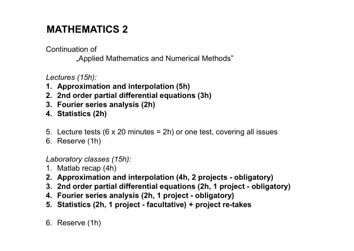
MATHEMATICS 2

Continuation of „Applied Mathematics and Numerical Methods” Lectures (15h):

• 1. Approximation and interpolation (5h)
• 2. 2nd order partial differential equations (3h)
• 3. Fourier series analysis (2h)
• 4. Statistics (2h)
• 5. Lecture tests (6 x 20 minutes = 2h) or one test, covering all issues
• 6. Reserve (1h)

Laboratory classes (15h):

• 1. Matlab recap (4h)
• 2. Approximation and interpolation (4h, 2 projects - obligatory)
• 3. 2nd order partial differential equations (2h, 1 project - obligatory)
• 4. Fourier series analysis (2h, 1 project - obligatory)
• 5. Statistics (2h, 1 project - facultative) + project re-takes
• 6. Reserve (1h)

APPROXIMATION AND INTERPOLATION

• General formulation
• Interpolation (monomials, Lagrange) – short review
• LS approximation (discrete, continuous)
• Chebyshev polynomials
• Orthogonal and orthonormal polynomials
• Spline interpolation

Y X

 

1 1, y

x

 

2 2, y

x

 

n n y

x ,

Continuous approximation

x a  x b 

   

p x y f x y   

 

y f x 

 

y p x 

Discrete approximation

   

1,2,...,

,

i i i n

x y y p x



 

Y X Interpolation: discrete approximation variant

 

y p x 

 

,

i i

x y

 

, 1,2,...,

i i

y p x i n  

Y X

 

y p x 

 

, ,

i i i

x y  

Processing of the experimental measurements (over-fitting phenomena)

Physically based approximation (optimal smooth solution)

 

, 1,2,...,

i i i

y p x i n    

Y

 

y p x 

 

, ,

i i i

x y  

Over-smoothing phenomena Y

 

y p x 

 

, ,

i i i

x y  

discrete type continuous type

   

1,2,...,

,

i i i n

x y y p x



 

 

 

 

, x a b

y p x x f y



  

1 1 1

( ) ( ) ... ( ) ( )

m m m j j j

p x a x a x x a   



    



unknown numbers (not functions) known (given) basis functions approximation: solution of system of linear algebraic equations (SLAE)

1 1 1

( ) ( ) ... ( ) ( )

m m m j j j

p x a x a x x a   



    



For continuous and discrete approximations:

 

1 2 1 2 ( 1) (1 )

( ) ( ) , : ( ) ( ) ( ) ... ( ) , ...

m m m m

a a p x x where x x x x a   

 

                a a  

n = m (interpolation, determined SAE) n > m (approximation, over-determined SAE) n < m (ill-posed problem, undetermined SAE) For discrete type: Basis functions:

( ) , 1,...,

j x

j m  

(linearly independent)

Interpolation (n = m)

1 1 1

( ) ( ) ... ( ) ( )

n n n j j j

p x a x a x x a   



    



interpolation conditions:

1 1 1

( ) , 1,..., ( ) ( ) ... ( ) ( )

i i n i i n n i j i j j

p x y i n p x a x a x x a   



      



1

( ) , , 1,...,

n j i j i j

x a y i j n 



  



SLAE

1 1 2 1 1 1 1 1 2 2 2 2 2 2 ( ) ( 1) ( 1) 1 2

, : ( ) ( ) ... ( ) ( ) ( ) ... ( ) , , ... ... ... ... ... ... ( ) ( ) ... ( )

n n n n n n n n n n n n

where x x x a y x x x a y x x x a y         

  

                                       Aa = B A a B

existence and uniqueness of the SLAE solution

, ( )

i j j

x x i j x   

linearly independent functions (nodes can not overlap) if so:

 

1

det ,



 A a = A B

the simplest case: monomials

1

( ) , 1,...,

j j x

x j n 



 

1 1 1 1 1 1 2 2 2 2 ( ) ( 1) ( 1) 1

, : 1 ... 1 ... , , ... ... ... ... ... ... 1 ...

n n n n n n n n n n n

where a y x x a y x x a y x x

     

                                         Aa = B A a B

2 1 1 1 2 3 1

( ) 1 ...

n n j n j j

p x a a x a x a x x a

  

         



Van der Monde matrix

Lagrange interpolation

 

  

1 1 2 1 1 1 1 1 1 2 2 2 2 2 2 1 ( ) ( 1) ( 1) 1 2 1

, : ( ) ( ) ... ( ) ( ) ( ) ... ( ) , , ... ... ... ... ... ... ( ) ( ) ... ( )

n n n n n n n n n n n n

where L x L x L x a y L x L x L x a y a y L x L x L x

  

                                                           Aa = B A a B

,

i i

a y    A = I Ia = B a = B

as the consequence:

 

( ) , 1,...,

j j

x L x j n   

 

, 1 ,

j i

i j L x i j      

       

1 1 2 2 1

( ) ...

n n n j j j

p x y L x y L x y L x y L x



       

Lagrange polynomials

1

x

2

x

3

x

 

1

L x

 

2

L x

y = 1

 

3

L x

Runge effect (remedy: approximation, nodes distribution, spline interpolation) good bad ?

approximation of discrete type (m < n)

   

1,2,..., 1

, ( ) ( )

i i i n m j j j

y x a p x x x y 

 

     



a 

approximation: fitting a curve to set of points best approximation: minimising the approximation error (using appropriate norm)

 

 

2 2 2 1 1

1 1

n n i i i i i

L e p x y n n

 

  

 

   

 

max

max max

i i i i i

L e p x y   

Least squares (LS) method:

 

2

min

j

a

L

min-max method

 

max

min

j

a

L

 

   

 

   

2 2

min min

T T

nL         

a a

Aa B Aa B Aa B Aa B a

 

T

  A Aa B

following the matrix (absolute) notation:

1

( )  

   

      a B a B 

1 1 2 1 1 1 2 2 2 2 1,..., ( ) 1,... 1 2

( ) ( ) ... ( ) ( ) ( ) ... ( ) ( ) ... ... ... ... ( ) ( ) ... ( )

m m i n j i n m j m n n m n

x x x x x x x x x x          

  

                  A

 

1 2 1,..., ( 1)

...

i i n n n

y y y y

 

              B

• r

1

,

T T 

   Ca D a C D , C = A A D A B 

following the index notation:

 

2 2 2 1 1 2 1 1 1 1

min ( ) ( ) 2 ( ) ( )

n m j i j i i j n m n m j i j i j i j i k i i j i j k

nL x a y x a y x a y x a    

     

                              

     

a

more accurate value

 

1,2,...,

,

i i i n

x y



 

1,2,...,

, ,

i i i i n

x y 



weights:

 

i i i i

e p x y      

 

   

2 2 2 2 1 1

min min ( ) ( )

n n i i i i i i i i

nL x y x y  

 

        

 

a a

a a a  

1

,

T T 

   Ca D a C D , C = A WA D A WB 

 

1 2 1,..., ( )

... ... ... ... ... ... ...

i i n n n n

diag    

 

              W

in case of two weight levels:

• low ( = 1)
• high ( = 10, 100, etc)
• nly m higher weights may be applied

how to make it smaller?

approximation of continuous typee

 

 

 

, 1

( ) ( )

m x b j a j j

y f x x a x y p x 

 

      



a  approximation: fitting a curve to set of points best approximation: minimising the approximation error (using appropriate norm)

   

 

2 2

1

b a

L p x f x dx b a    

     

max

max max

x x

L e x p x f x   

Least squares (LS) method:

 

2

min

j

a

L

min-max method

 

max

min

j

a

L

 

 

   

2 2 2 2

min min ( ) ( ) ( ) ( )

b b a a

b a L x f x dx x f x dx          

 

a a

a a a  

 

2 ( ) ( ) ( ) ( ) ( ) ( ) ( ) ( ) ( ) ( ) ( )

b b T T T a a b b T T a a

x x f x dx x x x f x dx x x dx x f x dx          

   

a a a        

1 

  Aa B a A B 

1 1 1 2 1 2 1 2 2 2 ( ) , 1,... 1 2

( ) ( ) ( ) ( ) ... ( ) ( ) ( ) ( ) ( ) ( ) ... ( ) ( ) ( ) ( ) ( ) ( ) ... ... ... ... ( ) ( ) ( ) ( ) ... (

b b b m a a a b b b b b T m a a a i j a a m m i j m b b m m m a a

x x dx x x dx x x dx x x dx x x dx x x dx x x dx x x dx x x dx x x dx x                   

 

         

         

A   ) ( )

b m a

x dx                   



1 2 ( 1) 1,...,

( ) ( ) ( ) ( ) ( ) ( ) ( ) ( ) ... ( ) ( )

b a b b b T a i a a m i m b m a

x f x dx x f x dx x f x dx x f x dx x f x dx    

 

                          

    

B  (easy) (difficult)

for monomial basis functions:

1 2 1 1 2 1 1

( ) ...

m j m m j m m j

p x a x a a x a x a x

    

     



1 1 1 ,

1 1

b p q p q p q b b p q p q i j a a a

x b a A x x dx x dx p q p q

      

         

 

1

( ) ( ) ( ) ... ( )

b a b b p a i a b m a

f x dx x f x dx B x f x dx x f x dx



                    

   

( ) , ( )

p q i j

x x x x    

troublesome (due to f(x) ), usually numerical integration required

numerical integration (division into k subintervals)

x a  x a t  

 

1 x a k t    x b 

1 k j

x a jt  

 

1 x a j t   

for trapezoidal rule: for Gaussian rule (2 points)

   

1 1 2 2 1

( ) , 1,2,..., 2

k b p p p i a j

t B x f x dx x f x x f x i m



         

 

 

1

2 2 1 2 2 3 a j t t x     

 

2

2 2 1 2 2 3 a j t t x    

b a t k  

   

1 1 2 2 1

( ) , 1,2,..., 2

k b p p p i a j

t B x f x dx x f x x f x i m



         

 

 

1

1 x a j t   

2

x a jt  

Are weights applicable in case of continuous approximation? weight function may control the accuracy in continuous manner (on the whole interval)

( ) y x   

smaller approx. error larger approx. error

( ) , 1,...

( ) ( ) ( ) ( ) ( ) ( )

b b T i j a a m m i j m

x x x dx x x x dx    

 

        

 

A  

   

( 1) 1,...,

( ) ( ) ( ) ( )

b b T i a a m i m

x f x x dx x f x x dx   

 

       

 

B 

Are weights applicable in case of continuous approximation?

1 1 1 2 1 2 1 2 2 2 ( ) 1 2

( ) ( ) ( ) ( ) ... ( ) ( ) ( ) ( ) ( ) ( ) ... ( ) ( ) ... ... ... ... ( ) ( ) ( ) ( ) ... (

b b b m a a a b b b m a a a m m b b m m m a a

x x dx x x dx x x dx x x dx x x dx x x dx x x dx x x dx x                 





       

                    A ) ( )

b m a

x dx                         



• rthogonal basis functions:

, ( ) ( ) ,

b i j a

i j x x dx i j         



• rthogonal (with weight) basis functions:

 

, ( ) ( ) ,

b i j a

i j x x x dx i j          



• rthonormal basis functions:

, ( ) ( ) 1 ,

b i j a

i j x x dx i j         



• rthonormal (with weight) basis functions:

 

, ( ) ( ) 1 ,

b i j a

i j x x x dx i j          



Example Given is

   

sin f x x 

in

0, 2 x       

. Find its

• discrete LS approximation (apply three nodes regularly spaced),
• weighted LS discrete approximation (apply  = 10 for the first node)
• continuous LS approximation
• continuous weighted LS approximation (apply (x) = x )

Apply Each time, evaluate the approximation error (as a function and a norm).

 

2 1 2

p x a a x  

   

sin f x x 

 

2

0.2110 0.3483 p x x  

 

2

0.0306 0.4343 p x x  

 

2

0.4782 0.2694 p x x  

 

2

0.3279 0.3754 p x x  

2nd approach to overcome Runge effect: optimal distribution of nodes    

 

10,10

sin , 8

x

f x x n

 

 

( ) max 1

( ) ( )

n n i i

x f x x 



  



estimation of the interpolation error Chebyshev problem: find min of max error

1 1 1

min max ( )

i

n i x x i

x x

   





Solution: the solution to the above problem are the roots of Chebyshew polynomials

Chebyshev polynomials

 

 

( ) cos 1 cos

m

T x m arc x   

iterative definition recursive definition

1 2 1 2

( ) 1 ( ) ( ) 2 ( ) ( ) , 3

m m m

T x T x x T x x T x T x m

 

            1 1 x    n = 1 n = 2 n = 3 n = 4 n = 5 n = 6

2 1 cos , 1,2,..., 1 1 2

i

i x i m m              

Formula for Chebyshev polynomials’ roots Orthogonality of Chebyshev polynomials

1 2 1

0, ( ) ( ) , 1 2 1 , 1

i j ij

i j T x T x I dx i j x i j  



               



1 1 x    Transformation between intervals:

, , 1,1 z a b x    1 : [( ) ( )] 2 x z z b a x b a      

2 ( ) : z b a z x x b a     

Example Given is

   

sin f z z 

in

0, 2 z       

. Find:

• approximation data with nodes as roots of fourth Chebyshev polynomial
• SLAE for interpolation method using Chebyshev polynomials

Apply

       

1 1 2 2 3 3

p z a T z a T z a T z   

     

0.8660 1.4656,0.9945 , 0.7854,0.7071 , 0.8660 0.1052,0.1050    

solution:

1 2 3

1 0.8660 0.5 0.9945 0.6022 1 1 0.7071 0.5135 1 0.8660 0.5 0.1050 0.1049 a a a                                               a

       

2 1 1 2 2 3 3 2

4 4 0.6022 1 0.5135 1 0.1049 2 1 1 0.3401 1.1881 0.0162 p z a T z a T z a T z z z z z                                       

y = sin(x)

0.5 1 1.5 0.1 0.2 0.3 0.4 0.5 0.6 0.7 0.8 0.9 1

Lagrange Chebyshev error = 0.0187 error = 0.0162 3 points – 2nd order

• 10
• 8
• 6
• 4
• 2

2 4 6 8 10

• 5
• 4
• 3
• 2
• 1

1 2 3 4 5

y = sin(x) Lagrange Chebyshev error = 5.3767 error = 1.0825 8 points – 7th order

• 15
• 10
• 5

5 10 15

• 30
• 20
• 10

10 20 30

y = sin(x) Lagrange Chebyshev error = 36.0440 error = 1.3704 12 points – 11th order

Orthogonality (with weight) of Chebyshev polynomials

1 2 3

1 0.8660 0.5 0.9945 1 1 0.7071 1.4143 1 0.8660 0.5 0.1050 a a cond a                                   

SLAE for Chebyshev interpolation:

1 2 3

1 1.4656 2.1480 0.9945 1 0.7854 0.6169 0.7071 15.8567 1 0.1052 0.011 0.1050 a a cond a                                 

SLAE for monomial interpolation:

1 2 1

0, ( ) ( ) , 1 2 1 , 1

i j ij

i j T x T x I dx i j x i j  



               



Generation of orthogonal (orthonormal) (with weight) basis functions

• Gramm – Schmidt method
• rthogonal basis functions:

, ( ) ( ) ,

b i j a

i j x x dx i j         



• rthogonal (with weight) basis functions:

 

, ( ) ( ) ,

b i j a

i j x x x dx i j          



• rthonormal basis functions:

, ( ) ( ) 1 ,

b i j a

i j x x dx i j         



• rthonormal (with weight) basis functions:

 

, ( ) ( ) 1 ,

b i j a

i j x x x dx i j          



scalar product

 

, ( ) ( )

b i j i j a

x x dx      



 

 

, ( ) ( )

b i j i j a

x x x dx         



Generation of orthogonal (orthonormal) (with weight) basis functions

• Gramm – Schmidt method

Algorithm 1.

   

1 1 1

g x t f x  

   

, 1,2,..., , ,

j

f x j m x a b  

2.

for orthogonal

   

12 1 1 1 1 1

, 1 , g g t f f  



  

1

1 t 

for orthonormal

     

2 2 1,2 1

g x f x g x    

     

2 1 2 1 1,2 1 1

, , , f g g g g g       

   

2 2 2

g x t g x   

for orthonormal

   

12 2 2 2 2 2

, 1 , g g t g g  



    

3.

       

3 3 1,3 1 2,3 2

g x f x g x g x       

     

3 1 3 1 1,3 1 1

, , , f g g g g g       

   

3 3 3

g x t g x   

for orthonormal

   

12 3 3 3 3 3

, 1 , g g t g g  



    

     

3 2 3 2 2,3 2 2

, , , f g g g g g       

Generation of orthogonal (orthonormal) (with weight) basis functions

• Gramm – Schmidt method

   

, 1,2,..., , ,

j

f x j m x a b  

General formula

         

1 , 1

/

p p p i p i j i

g x f x g x x g x  

 

   



     

 

   

,

1 , 1 , ,

, , , , , 1,2,..., , 1,2,..., 1 ,

j p j j

p p j p j i p i j i g g p j j p j j

g g f g g g f g p m j p g g

 

      

  

      



    

for all cases

   

   

12

, , 1 ,

p p p p p p p p

g x t g x g g t g g  



       

for orthonormal (with weight) case

Example Given is

 

1

, 1,2,3 , 0, 2

i i

f x x i x 



       

• orthogonal series
• orthonormal series with weight
• use orthogonal series as basis functions for SLAE from previous example

 

x x  

Solution:

           

1 1 2 2 2 2 2 3 2 2 3

1 1 4 12 2 4 2 24 g x f x f x x g x x f x x g x x x x x                          

1 2 3

1 0.6802 0.2571 0.9945 1 0.2056 0.7071 4.6358 1 0.6802 0.2571 0.1050 a a cond a                                   

• 4
• 2

2 4 6 8 10

• 4
• 2

2 4 6 8 10 12

Interpolation using spline functions

• 4
• 2

2 4 6 8 10

• 4
• 2

2 4 6 8 10 12

Construction of quadratic spline

   

2 1 2 3

s x p x a x a x a    

     

2 2 2

s x p x b x x



  

 

1 1

, x y

 

2 2

, x y

 

3 3

, x y

 

,

n n

x y

       

2 2 2 2 3 3

s x p x b x x b x x

 

    

 

1 2 2

( ) ( )

n i i i

s x p x b x x

  

  



Basic data:

( , ), 1,2,...,

i i

x y i n 

1 1 2 1 1 2 1 1

( ) ...

k k k k i k k i i

p x a x a x x a a a x

      

         

spline on the 1st interval

1 2

, x x x 

1 1 1 1 2 1 2 i i

( ) ( ) ( ) ( ) ( ) , x > x , ( ) 0, x x

n k n k k i k i i i i i i i i k k i i

s x p x b x x a x b x x x x for x x for

          

            

  

 

1 1 2 2

( ) ( )

n i i i p x

s x a x a b x x

  

   



    

1 2 2 1 2 3 2 ( )

( ) ( )

n i i i p x

s x a x a x a b x x

  

    



   

 

1 3 2 3 1 2 3 4 2

( ) ( )

n i i i p x

s x a x a x a x a b x x

  

     



  

.

linear spline (2 + n - 2 = n unknows) quadratic spline (3 + n - 2 = n+1 unknows) cubic spline (4 + n - 2 = n+2 unknows) spline on

• ther intervals

Construction of the k-th order spline

• 4
• 2

2 4 6 8 10

• 4
• 2

2 4 6 8 10 12

Additional data for quadratic spline

 

1

' f x  

 

1 1

, x y

 

2 2

, x y

   

2 1 2 3

s x p x a x a x a    

• 4
• 2

2 4 6 8 10

• 4
• 2

2 4 6 8 10 12

Additional data for cubic spline

 

1 1

' f x  

 

1 1

, x y

 

2 2

, x y

 

,

n n

x y

 

1 1

,

n n

x y

 

 

'

n n

f x  

   

3 2 1 2 3 4

s x p x a x a x a x a     

• 4
• 2

2 4 6 8 10

• 4
• 2

2 4 6 8 10 12

Additional data for cubic spline

   

1 1

' '' f x f x         

 

1 1

, x y

 

2 2

, x y

 

,

n n

x y

 

1 1

,

n n

x y

 

   

3 2 1 2 3 4

s x p x a x a x a x a     

Determination of p(x) (parameters a)

1 1 1 1 1 1 2 1 1 1 2 2 1 2 2 2 2 2 2 2

( ) 1 ... ( ) 1 ... a y s x y a x a y x a s x y a x a y x a a y                                          linear spline

1 

   Aa B a A B

quadratic spline

2 2 1 1 1 1 1 1 2 1 3 1 1 1 1 2 2 2 2 1 2 2 2 3 2 2 2 2 2 2 1 1 1 2 1 3 3

( ) 1 ... ( ) 1 ... ( ) 2 2 1 ...

I

a y s x y a x a x a y x x a s x y a x a x a y x x a y a s x a x a x a a                                                                  

cubic spline

3 2 3 2 1 1 1 1 1 1 1 2 1 3 1 4 1 1 1 1 3 2 3 2 2 2 2 2 1 2 2 2 3 2 4 2 2 2 2 2 2 1 3 1 1 2 1 3 1 1 1 4 1 1 2 1

( ) ... 1 ( ) 1 ( ) 3 2 3 2 1 ( ) 6 2 6 2

I II

a y s x y a a x a x a x a y x x x a s x y y a x a x a x a y x x x s x a a x a x a x x s x a a x a x                                                                  

2 3 4

... ... ... a a a                        

Determination of parameters b

3 3 3 3 2 3 2 3 2 3 2

( ) ( ) ( ) ( ) ( )

k k

y p x s x p x b x x y b x x        

 

3 3

, x y

for  

4 4

, x y

for

4 4 2 4 2 4 4 2 4 2 3 4 3 4 3 4 3

( ) ( ) ( ) ( ) ( ) ( ) ( )

k k k k

y p x b x x s x p x b x x b x x y b x x            

… for

1,

2,3,..., 1

j

x x j n



  

1 1 1 1 2 1 1 1 1 1 2

( ) ( ) ( ) ( ) ( ) ( )

j k j j i j i j i j k k j i j i j j j j i

s x p x b x x y p x b x x b x x y

          

          

 

1 1 1 1 2 1

( ) ( ) , 2,3,..., 1 ( )

j k j j i j i i j k j j

y p x b x x b j n x x

     

      



Example Given is the set of points: x y 0 1 2 3 1 3 8 Find quadratic spline, assume y’(0) = 0              

2 2 2 2 2 2 2

, 1 1 2 1 , 1 2 1 3 2 3 10 11 , 2 3 x x s x x x x x x x x x x x                      

2nd ORDER PARTIAL DIFFERENTIAL EQUATIONS

• Classification
• Elliptic equations: local and global (variational) formulations
• Fundamentals of FDM (finite difference method)
• Laplace and Fourier elliptic equations
• Parabolic equations: explicit and implicit time formulas
• Hyperbolic equations

Classification

2 2 2 2 2

, u u u u u a b c d e g u f a b c x x y y x y                        unknown function

 

, u u x y 

, , , , , , a b c d e f g

known coefficients: functions or numbers

 

 

, x y  

problem domain

2

4 b ac     

elliptic type parabolic type hyperbolic type

   

Equation type may change within Ω

Elliptic equations

Examples: static analysis in elastic range (plane stress, plane strain, bar torsion) stationary heat flow analysis filtration through the porous system distribution of the magnetic and electric charges

b

(0)

t

(0)

u

u









 

linear elasticity



T



q



n

q

heat flow analysis

natural (Neumann b.c.) essential (Dirichlet b.c.)

f

Heat flow analysis

   

2 2 2 2

,

t x y x T T t y q n q x y

T T T T T k k f in x y T f in x y k T T

• n

T T

• n

k T T q

• n

k q

• n

n n n                                                                       D D n D n

local formulation

2

T C 

variational formulation

   

 

     

1

, , , , , ,

q

t

v x y T x y d v x y f x y d v x y qd v H

  

      

  

  D

find such

1 1

T H H T   

     

1

, , , ,

q

x y

v T v T k k d v x y f x y d v x y qd v H x x y y

  

               

  

a good start for most of the computational approaches (FEM, variational (M)FDM) (a good start for local / standard (M)FDM)

Example Given is the differential equation

   

1 1 , 2

xx xy yy x

u a u u u f x y     

Problem domain constitutes the figure limited by:

• the bottom right quarter of the circle
• the skew line
• the horizontal straight line y = 0.

Along the semicircle and skew line, natural b.c. are ascribed, along the horizontal line – essential b.c.

• determine such values of parameter a that

the above equation remains elliptic.

• determine the right hand side function f(x, y)

knowing the solution of this equation is

• write the b.c.: essential and natural ones for any point (x, y)

 

2 2

, u x y x y  

2 2

1 x y   1 y x   

Finite difference method (FDM) recap

difference operators: replacement of the analytical derivatives with numerical ones x

 

y f x 

1D:

i

x

   

' , ''

i i

f x f x h

i

y

1 i

y 

1 i

y 

1 1 1 1 1 1 2

' 2 2 ''

i i i i i i i i i i i

y y h y y y h y y h y y y y h

     

               

2D: formulas composition

i

x

1 i

x  h

1 i

x 

FD star FD formulas, FD schemes FD operators:

xx yy

T T  

1 1 1 1

• 4

2

1 h 

h h h h

x

Example



2 2 2 2

2

C

F F G in x y F

• n

              

 

5a 3a

h a 

1 2 Generate FD system of equations, by means of the:

• local formulation
• variational formulation

Use matrix form of SLAE.

1

, , v F v Fd C v d F v H x x y y

 

             

 

prismatic bar torsion F – Prandtl function

2 2

, ,

zx zy z zx zy

F F y x              

Dealing with natural b.c. in FDM, evaluating stresses

• > Computational methods in civil engineering

Parabolic equations

Examples: diffusion non-stationary heat flow analysis

 

, , , ,

xx t

u u f x t a x b t t        

 

, u u x t 

unknown temperature function

 

, f f x t 

intensity of heat generation inside the domain boundary conditions

       

, ,

a b

u a t u t u b t u t       

initial condition

   

, u x t u x 

x t

 

u x a b

 

a

u t

 

b

u t  a b x  t 

a) problem formulation b) FD discretization

t

Parabolic equations

xx t

u u f    

unknown level known level

,

k

k t

1

1,

k

k t  

1, i k  , i k 1, i k  1, 1 i k   , 1 i k  1, 1 i k  

x  x  t 

unknown level known level

,

k

k t

1

1,

k

k t  

1, i k  , i k 1, i k  , 1 i k 

x  x  t 

the simplest approach: three nodes at known level, one node at unknown level

 

1, , 1, 2 ,

2

i k i k i k xx i k

u u u u x

 

   

Numerical approximation of the 2nd space derivative: Numerical approximation of the 1st time derivative:

 

, 1 , , i k i k t i k

u u u t

 

 

After substitution into differential equation :

1, , 1, , 1 , , 2

2

i k i k i k i k i k i k

u u u u u f x t 

  

      

xx t

u u f    

where:

 

,

, , ...

i k i k

u u x t 

 

,

,

i k i k

f f x t 

2

t x     

One constant instead of three ones:

 

, 1 1, , 1, ,

1 2

i k i k i k i k i k

u u u u t f   

  

      

Final form:

 

, 1 1, , 1, ,

1 2

i k i k i k i k i k

u u u u t f   

  

      

1 2  

Explicit, open scheme conditionally stable

2

1 2

crit

x t t      

unknown level known level

,

k

k t

1

1,

k

k t  

1, i k  , i k 1, i k  , 1 i k 

x  x  t 

leads to one value at time (no SLAE) λ λ 1

1-2λ

, i k

t f  

t  x  x 

unknown level known level

,

k

k t

1

1,

k

k t  

1, i k  , i k 1, i k  1, 1 i k   , 1 i k  1, 1 i k  

x  x  t 

unknown level known level

,

k

k t

1

1,

k

k t  

, i k , 1 i k 

x  x  t 

more complex approach: three nodes at unknown level, one node at known level

1, 1 i k   1, 1 i k  

 

1, 1 , 1 1, 1 2 , 1

2

i k i k i k xx i k

u u u u x

     

   

Numerical approximation of the 2nd space derivative: Numerical approximation of the 1st time derivative:

 

, 1 , , 1 i k i k t i k

u u u t

 

  

After substitution into differential equation :

1, 1 , 1 1, 1 , 1 , , 1 2

2

i k i k i k i k i k i k

u u u u u f x t 

      

      

xx t

u u f    

where:

 

, 1 1

, , ...

i k i k

u u x t

 



 

, 1 1

,

i k i k

f f x t

 



2

t x     

One constant instead of three ones:

 

1, 1 , 1 1, 1 , 1 ,

1 2

i k i k i k i k i k

u u u t f u   

     

       

Final form:

 

1, 1 , 1 1, 1 , , 1

1 2

i k i k i k i k i k

u u u u t f   

     

       

t    

Simple implicit, closed scheme unconditionally stable leads to SLAE at each time level unknown level known level

,

k

k t

1

1,

k

k t  

, i k , 1 i k 

x  x  t 

1, 1 i k   1, 1 i k  

• λ
• λ

1

1+2λ

, 1 i k

t f



 

t  x  x 

unknown level known level

,

k

k t

1

1,

k

k t  

, i k , 1 i k 

x  x  t 

1, 1 i k   1, 1 i k  

Crank – Nicolson scheme

 

     

1, 1 1, , 1 , 1, 1 1, 2 , 1

1 1 1 2 2 2 2

i k i k i k i k i k i k xx i k

u u u u u u u x

       

      

   

1, , 1, 1, 1 , 1 1, 1 , 1

1 1 2 2 2 2

i k i k i k i k i k i k i k

u u u u u u t f      

       

           Complex implicit, closed scheme, unconditionally stable

Example

       

, , , 4 , 0, 10 (4, ) 10 ,0 4 10

xx t

u u x t x t u t u t u x x x                Assume 5 nodes at each time level, as well as the time step, being the half of the critical time step. Perform calculations for two time steps. Apply explicit and implicit time schemes. Use symmetry conditions, if available. Solve the equation:

Hyperbolic equations

Examples: forced bar vibrations problems of theory of plasticity

 

, , , ,

xx tt

u u f x t a x b t t       

 

, u u x t 

unknown deflection function

 

, f f x t 

mass forces boundary conditions

       

, ,

a b

u a t u t u b t u t       

initial conditions

       

, ' ,

t

u x t u x u x t v x       

E    

x t

   

, u x v x a b

 

a

u t

 

b

u t  a b x  t 

a) problem formulation b) FD discretization

t

Hyperbolic equations

xx tt

u u f   

unknown level

,

k

k t

1

1,

k

k t  

1, i k  , i k 1, i k  1, 1 i k   , 1 i k  1, 1 i k  

t 

1

1,

k

k t  

1, 1 i k   , 1 i k  1, 1 i k  

x  x  t 

known level known level unknown level known level

,

k

k t

1

1,

k

k t  

1, i k  1, i k 

x  x  t 

1

1,

k

k t  

known level

t 

, i k , 1 i k  , 1 i k 

Numerical approximation of the 2nd space derivative: Numerical approximation of the 2nd time derivative: After substitution into differential equation :

1, , 1, , 1 , , 1 , 2 2

2 2

i k i k i k i k i k i k i k

u u u u u u f x t 

   

       

xx tt

u u f   

where:

 

,

, , ...

i k i k

u u x t 

 

,

,

i k i k

f f x t 

2 2

t x     

One constant instead of three ones:

 

2 , 1 1, , 1, , 1 ,

2 2

i k i k i k i k i k i k

t u u u u u f    

   

      

Final form:

 

1, , 1, 2 ,

2

i k i k i k xx i k

u u u u x

 

   

 

, 1 , , 1 2 ,

2

i k i k i k tt i k

u u u u t

 

   

 

2 , 1 1, , 1, , 1 ,

2 2

i k i k i k i k i k i k

t u u u u u f    

   

      

1  

Explicit, open scheme conditionally stable

kryt

t t x      

leads to one value at time (no SLAE) λ λ 1

2 , i k

t f   

t  x  x 

• 1

t 

2-2λ

unknown level known level

,

k

k t

1

1,

k

k t  

1, i k  1, i k 

x  x  t 

1

1,

k

k t  

known level

t 

, i k , 1 i k  , 1 i k 

Example

         

4 , , , 4 , 0, (4, ) ,0 4 ,0

xx tt

u u x t x t u t u t u x x x v x                  Assume 5 nodes at each time level, as well as the time step, being the half of the critical time step. Perform calculations for two time steps. Apply explicit time

• scheme. Use symmetry conditions, if available.

Solve the equation (forced bar vibrations):

Fourier series analysis

• General formulation for periodic function
• General formulation for function in arbitrary interval
• Beam deflection problem
• Bending plate problem

Motivation

Fourier analysis:

• representation of the wave-like functions as the simple sin
• r / and cos functions
• decomposition of any periodic function / signal into a finite sum of simple
• scillating functions

Applications:

• function approximation method,
• harmonic analysis (frequencies, periods, amplitudes),
• noise filtering, signal processing
• „exact” analytical solution of boundary value problems.

General formulation (periodic function)      

 

1

cos sin 2

k k k

a f x a kx b kx

 

  



For any periodic function with period 2π Trigonometric base fulfils the orthogonality properties

               

cos sin sin cos , , sin sin , , cos cos , 2 , kx dx kx dx k kx mx dx k m k m kx mx dx k m k m kx mx dx k m k m

         

  

    

                       

    

 

 

x    

General formulation

In search of coefficients ak and bk

     

 

 

cos sin / cos

k k k

f x a kx b kx mx

 

  



   

, cos cos , 2 , k m kx mx dx k m k m

 

 



          



   

cos f x mx dx

  

           

1 1 cos 0 , cos , 1,2,... 1 cos , 0,1,2,...

k k

a f x x dx a f x kx dx k a f x kx dx k

     

  

  

     

  

General formulation

In search of coefficients ak and bk

     

 

 

cos sin / sin

k k k

f x a kx b kx mx

 

  



   

, sin sin , k m kx mx dx k m

 





     



   

sin f x mx dx

  

   

1 sin , 1,2,...

k

b f x kx dx k

 

   



General formulation (arbitrary function)  

1

cos sin 2

k k k

a k x k x f x a b L L  

 

                    



For function in arbitrary interval:

 

x L L  

 

1 cos

L k L

k x a f x dx L L 



      



 

1 sin

L k L

k x b f x dx L L 



      



For even functions: For odd functions:

k

b 

k

a 

 

x a b 

 

1 , 2

b a

b a L dx L  

 

For which functions their Fourier series are convergent to them?

Dirichlet theory If y = f(x), bounded on interval [-L, L], is:

• 1. Monotonic in subintervals inside [-L, L],
• 2. Continuous in [-L, L], expect for finite number of discontinuity points of the

first order

• 3. Function f(x) has finite number of local minima and maxima in [-L, L].
• 4. Values at both interval ends should be the same

   

lim , lim

x x x x

f x f x

 

 

   

Additionally if y = f(x) is periodic and its period is 2L, then its development holds for all x

   

f L f L  

Examples

       

sin 2cos 3 5sin 7 f x x x x   

a= -0.0000 0.0000

• 2.0000

0.0000

• 0.0000
• 0.0000
• 0.0000
• 0.0000

0.0000 0.0000 0.0000

• 0.0000

0.0000 b= 1.0000

• 0.0000
• 0.0000
• 0.0000

0.0000

• 0.0000

5.0000

• 0.0000
• 0.0000
• 0.0000

0.0000

• 0.0000

0.0000 a0=-2.9155e-16

n = 13

Examples

           

2

sin 2cos 3 5sin 7 (cos 47 sin 32 ) f x x x x x x x       

a= -0.0016 0.0016

• 2.0016

0.0016

• 0.0016

0.0017

• 0.0017

0.0017

• 0.0017

0.0018

• 0.0018

0.0019

• 0.0020

b= 0.9997 0.0005

• 0.0008

0.0010

• 0.0013

0.0016 4.9981 0.0023

• 0.0026

0.0031

• 0.0035

0.0040

• 0.0046

a0 = 0.0016

n = 13

Examples

n = 5 n = 10 n = 15 n = 20

 

2

f x x 

Examples

n = 5 n = 10 n = 15 n = 20

Simply supported beam deflection problem

 

q x , L EJ

 

4 4

q x d y dx EJ 

static relations

 

3 3

T x d y dx EJ 

 

2 2

M x d y dx EJ  

distributed load, differential equation shear force bending moment

 

y x

       

2 2 2 2

y y L d y d y L dx dx         

Procedure

• 1. Formulate distributed load as the Fourier series
• 2. Substitute the above formulas into differential equation

   

1

2 sin , sin

L n k k k

k x k x q x q q q x dx L L L  



             

 

Main idea

 

1

sin

n k k

k x y x y L 



       



Simply supported beam deflection problem

a-priori fulfillment of the boundary conditions

 

4 4

q x d y dx EJ 



4 4 4 1 1

1 sin sin

k

n n k k k k

k k x k x y q L L EJ L



  

 

            

 

• 3. Evaluate coefficients yk
• 4. Compose solution and its derivatives

4 4 4

, , , 1,2,...,

k k k k k k

q k EJ y k n L         

 

1

sin

n k k

k x y x y L 



      



 

2 2 2 1

sin

n k k

k x M x EJ k y L L  



      



 

3 3 3 1

cos

n k k

k x T x EJ k y L L  



       



deflection bending moment shear force

numerical integration (division into m subintervals)

x  x h 

 

1 x k h   x L 

1 m j

x j h 

 

1 x j h  

for Simpson rule:

L h m 

3 1 2 1 2 3 1

2 ( )sin 1 ( ) sin 4 ( ) sin ( ) sin , 1,2,..., 3

L k m j

k x q q x dx L L k x k x k x h q x q x q x k m L L L L    



                                      

 

 

1 2 1 3 1

1 , , 2 h x j h x x x x h      

   

1

2 sin , sin

L n k k k

k x k x q x q q q x dx L L L  



             

 

Numerical integration for arbitrary type of load

, L EJ

Simply supported beam with constant load

q , L EJ

 

y x

 





1 1 1 ,

• dd

1 , even

sin 2 2 sin cos 4 ,

• dd

2 cos cos0 , even

n k k L L k k k

k x q x q L q q k x L k x q dx L L L k L q k q k k k k       

 

                                         

 

  

4 4

q d y dx EJ 

Simply supported beam with constant load

n = 1, k = 1 (error = 3.2%) (18.94%) L=10m q=10 kN/m EJ=10^6 kNm2

2 2 2 2 3

1 0.125 8 4 0.129

true Fourier

M q L q L M q L q L     

2

0.5 4 0.4053

true Fourier

T q L T q L q L    

4 4 4 4 5

5 0.0130 384 4 0.0131

true Fourier

q L q L y EJ EJ q L q L y EJ EJ     

(error = 0.48%)

Simply supported beam with constant load

n = 15, k = 15

• max. error = 0.0005%

125; 124.97 (0.02%) 50 48.91 (2.18%) L=10m q=10 kN/m EJ=10^6 kNm2

Simply supported beam with constant piecewise load

q , L EJ

 

y x

 

1 2 2 2 2

sin 2 2 2 2 sin sin cos cos 2 2 2 cos 1 cos cos cos 2cos 1 2 2 2

n k k L L L L k L L

k x q x q L q q q q k x k x L k x L k x q dx dx L L L L L k L L k L q q q k k k k k k k k               



                                                              

  

q

4 4

1 , 2 1 , 2 L x q d y L dx EJ x          

Simply supported beam with constant piecewise load

n = 2, k = 2 L=10m q=20 kN/m EJ=10^6 kNm2

Simply supported beam with constant piecewise load

n = 15, k = 1 L=10m q=20 kN/m EJ=10^6 kNm2

, L EJ

 

y x

Simply supported beam with concentrated force

P

4 4

2 d y P L x dx EJ         

 

1

sin 2 2 2 2 sin sin sin 2 2

n k k L k

k x q x q L L k P L k x P P k q x dx L L L L L     



                                      

 

Dirac delta properties:

   

d H x x x x dx    

     

f x x x dx f x 

 

 



selective property

n = 2, k = 2 L=10m, P=10 kN, EJ=10^6 kNm2 n = 1 n = 10 n = 20 n = 50

Bending rectangular plate

load as the Fourier sum deflection as the Fourier sum differential equation

(all formulas taken from the handouts written by dr M.Jakubek)

After substitution of deflection function and load function into differential equation Deflection coefficients Post processing

Bending rectangular plate – uniform load

m or n is even m and n are odd

Bending rectangular plate – concentrated force

plate subjected to concentrated force a = 2 m n = m = 50 v = 0.3 E = 20*10^6 kN/m2 P = -1000 kN h = 0.2 m x0 = y0 = a/2 = 1 m plate subjected to uniform load a = 2 m n = m = 50 v = 0.3 E = 20*10^6 kN/m2 q = -1000 kN/m h = 0.2 m

maximum deflection convergence with respect to the number

• f Fourier series – uniform load

maximum deflection convergence with respect to the number

• f Fourier series – concentrated force

Elements of „applied” probability

• Deterministic vs. probabilistic approaches
• Fuzzy logic – data and results randomness
• Monte Carlo simulations for integration
• Monte Carlo + random walk for differential equations
• Genetic algorithms for optimization and inverse problems

Deterministic vs. probabilistic approaches

Deterministic approach

• ne set of data parameters (geometry, load, material parameters, …)
• usually average values
• ne unique solution

methods : FEM, FDM, meshless methods, … Probabilistic approach variety of sets of data parameters, each with different prescribed stochastic (probability) family of solutions methods: soft computing (Monte Carlo simulations, genetic algorithms, artificial neural networks) + FEM, FDM, meshless methods

Application of probabilistic approaches

In mathematics:

• integration (in many dimensions)
• analysis of differential and integral equations

In civil engineering:

• influence of data parameters variability on the solution sensibility
• determination of reliability of a structure (probability that the failure state

does not appear)

• optimization problems (the optimal load / supports position that minimizes

e.g. the total potential energy)

• inverse problems (known is the answer, unknown are the parameters)

FUZZY SETS Membership functions

1

(1.5,2.5) x 

2

(2.5,3.5) x 

Boundary value problem (beam deflection) with fuzzy data (variable concentrated force and moment positions)

''( ) ( ), (0,4) (0) (4) u x f x x u u    

1

(1.5,2.5) x 

2

(2.5,3.5) x 

1

(1.5,2.5) x 

2

(2.5,3.5) x 

1   0.67   0.33    

FUZZY SETS (cont.)

fuzzy model for beam deflection fuzzy model for deflection in the middle 3D view - membership function for beam deflection FUZZY SETS (cont.)

s



f



safe failure

( ) p x

f



Reliability of structure

max adm

g w w  

max

w

• maximum deflection

adm

w

• admissible deflection

safe location failure location

max

w

adm

w

failure solution safe solution

g         g    

Reliability estimation

( ) ( )

f f s

f f

p x d n P n p x d

  

     

 

Probability of failure

f

n

• number of failures

n

• number of simulations

1

f

n n R P n    

safe Engineering application: reliability estimation

simulation Bending moment Beam deflection failure safe safe

adm

w w M ( ) p x x

Engineering application: reliability estimation (cont.)

mean values number of simulations

5

2000 100 2 10 n simulations series    

singular simulation exact value Reliability Engineering application: reliability estimation (cont.)

Monte Carlo method - introduction Stanisław Ulam (13.04.1909 – 13.05.1984) works:

• Manhattan project (1943 – 1967): contraction theory of

the hydrogen bomb

• creator of Monte Carlo method
• numerical methods, algorithms, informatics (ENIAC)

John von Neumann (28.12.1903 – 8.02.1957) works:

• Manhattan project (1943 – 1967): construction theory
• f the hydrogen bomb
• creator of games theory, cell automata
• quantum mechanics, informatics (ENIAC)

Introductory example – π evaluation

• 1. Definition of the input domain
• 2. Random generation of n INPUT DATA
• 3. Evaluation of a number of „FITTING” DATA („successes”)

 

2 2 2

, , , x y r x y r r    

   

, , , 1,...,

i i

x y r r i n   

2 2 2

1,...,

s i i

n x y r i n    

s

n

• 4. Evaluation of final results

2

4

s s circle square

n n Area Area r n n    

for r = 1 :

4

s

n n   

1D MC integration x y

max

f ( ) y f x  x a  x b 

 

max f

n P f b a N  

   

max

, , 0, , 1,...,

i i

x a b y f i N   

1D MC integration – results for MISER MONTE CARLO

 

( ) sin( ) cos( ) , 2,10 y x x x x x    

1D MC integration – results for VEGAS MONTE CARLO

 

( ) sin( ) cos( ) , 2,10 y x x x x x    

Laplace differential equation: Monte Carlo + random walk

'' ''

xx yy

F F in F x y

• n

      1 4 F n  

x y 4

2 10 F n   3 6 F n   6 5 F n   7 9 F n   8 6 F n   3 3 F n   2 12 F n   1 5 F n   8 3 F n   7 11 F n   6 6 F n  

4

   

1 2,2 4 20 18 36 77 24 30 63 48 5 24 9 4.48 , 12% 80 F e              

n = 80 random walks for x = 2, y = 2

Laplace differential equation: Monte Carlo + random walk

   

 

1, 1, , 1 , 1 , 2 , 1, 1, , 1 , 1 , ,

1 4 , ,

i j i j i j i j i j i j i j i j i j i j i j r s r s r s

F F F F F h F F F F F for x y F F for x y

       

                   1 1 1 1 4 4 4 4

h h j+1 j j-1 i-1 i i+1 i+1

 

 

, 1, 1, , 1 , 1 , ,

, ,

i j i j i j i j i j i j r s r s r s

E E E E E for x y E F for x y

   

            1 1 1 1 4 4 4 4

Laplace differential equation: Monte Carlo + random walk

'' ''

xx yy

F F in F F

• n

    

1

1

boundary

N i i i

F n F n



 



n = 10000

Laplace differential equation: Monte Carlo + random walk

MC solution = 3.341 FDM solution = 3.333 exact solution = 3.333

 

 

'' '' , , 0 3 , 0 3 ( , )

xx yy

F F in x y x y F x y x y

• n

          

Laplace differential equation: Monte Carlo + random walk

 

 

'' '' , , 0 3 , 0 3 ( , )

xx yy

F F in x y x y F x y x y

• n

           30 x 30 nodes

Poisson differential equation: Monte Carlo + random walk

     

 

( , ) 3 3 '' '' ( , ) , , 0 3 , 0 3 ( , )

xx yy

u x y x x y y F F f x y in x y x y F x y

• n

            

 

2 , 1 1

1 ,

j

m N i j k k p k

F f x y h N

 

  



Poisson differential equation: Monte Carlo + random walk

 

 

2 2

( , ) '' '' ( , ) , , 0 3 , 0 3 ( , )

xx yy

u x y x y F F f x y in x y x y F x y F

• n

           

 

2 , , , , 1 1

1 ,

brzeg j

n m N i j r s r s k k r s p k

F F N f x y h N

 

          

 

   

 

( , ) 9sin 3 '' '' ( , ) , , 0 3 , 0 3 ( , )

xx yy

u x y x y F F f x y w x y x y F x y F na                   

Poisson differential equation: Monte Carlo + random walk

Optimization

• 1. „brute force” (searching method)

number of target function values = 601 result accuracy = 0.002

• 2. bisection method (gradient method)

iteration number = 24 number of target function values = 72 results accuracy = 7e-7

• 3. feasible directions method
• 4. genetic algorithms (non gradient

method)

Genetic algorithms

Formulation:

) ( max s F

 

0,1

n

s 

Initial population:

 

  

M

s s s S ,..., ,

1

Generations:

N

S S S    ...

1

Three basic genetic operations:

• selection
• crossing
• mutation







M j j i i

s F s F p

1

) ( ) (

2 1

) 1 1001 1 10 (

m m

2 1

) 1 0101 1 11 (

m m

0,6 ≤ pc ≤ 0,9 M n pm    ) 1 ( 1 0 -> 1, 1 -> 0

 

2

max ( ) 15 F x x for x  

Let us assume 4-BITS strings (n = 4) , population size M = 4

member 1: 0 1 0 1 5 25 member 2: 1 0 0 1 9 81 member 3: 0 0 0 1 1 1 member 4: 1 0 0 0 8 64

INITIAL POPULATION S0: x F(x)

Fmax = 81, for x = 9 Fsum = 171 Fav = 42.75 Genetic algorithms – 1D example

Genetic algorithms – 1D example

SELECTION

member 1: 0 1 0 1 0.15 1 member 2: 1 0 0 1 0.47 2 member 3: 0 0 0 1 0.01 member 4: 1 0 0 0 0.37 1

p wheel of fortune selection

m 2 m 4 m 1 m 3

Population after selection

member 1: 0 1 0 1 5 25 member 2: 1 0 0 1 9 81 member 3: 1 0 0 1 9 81 member 4: 1 0 0 0 8 64

x F(x)

Fmax = 81, for x = 9 Fsum = 251 Fav = 62.75

Genetic algorithms – 1D example

CROSSING ( p = 0.9 )

member 1: 0 1 0 1 2 3 member 2: 1 0 0 1 3 4 member 3: 1 0 0 1 2 3 member 4: 1 0 0 0 3 4

m1 m2 Population after crossing

member 1: 0 0 0 1 1 1 member 2: 1 0 0 0 8 64 member 3: 1 1 0 1 13 169 member 4: 1 0 0 1 9 81

x F(x)

Fmax = 169, for x = 13 Fsum = 315 Fav = 78.75

Genetic algorithms – 1D example

MUTATION ( p = 0.2 )

member 1: 0 0 0 1 NNNN member 2: 1 0 0 0 NYNN member 3: 1 1 0 1 NNYN member 4: 1 0 0 1 NNNY

p Population after mutation

member 1: 0 0 0 1 1 1 member 2: 1 1 0 0 12 144 member 3: 1 1 1 1 15 225 member 4: 1 0 0 0 8 64

x F(x)

Fmax = 225, for x = 15 Fsum = 434 Fav = 108.5

Genetic algorithms – 1D example

Initial population

 

6 x sin(3 )cos( ) y x x 

Genetic algorithms – 1D example

Final population

 

6 x sin(3 )cos( ) y x x 

sin(10 ) 1 y x x   

 

1 2 x 

Initial population

Genetic algorithms – 1D example

 

1 2 x  sin(10 ) 1 y x x   

Number of target function values = Generations number x members number i.e. 100 x 20 = 2000

Final population

Genetic algorithms – 1D example

strain measurements

Inverse problems – truss example

OPTIMIZATION PROBLEM FORMULATION

TARGET FUNCTION

2 , , 1 ,

1 1

L i meas i calc i i meas

F L   



         



DECISION VARIABLES (n – problem size)

   

1 2 max

, ,..., , , 1,2,...,

n i

P P P P P i n  

L – number of bars with strain measurements OPTIMIZATION

 

1 2

, ,...,

max

n

P P P F

Inverse problems – truss example

measured strain at i-th bar (given value – measurement) calculated strain at i-th bar (by means of FEM algorithm)

GA + FEM algorithm

• BARS DIVISION

(BAR = FINITE ELEMENT)

• NUMBERING OF NODES, ELEMENTS, D.O.F.
• TOPOLOGY AND INCIDENT GENERATION

LOOP OVER ELEMENTS:

• STIFFNESS MATRIX GENERATION
• STIFFNESS MATRIX GENERATION
• NUMBER OF VARIABLES ASSUMED
• DETERMINATION OF STRINGS LENGTH

AND BITS NUMBER

• GENERATION OF INITIAL POPULATION

(FORCES)

• APPLYING FOR BOUNDARY CONDITIONS
• MATRIX ELIMINATION
• FEM PROBLEM SOLUTION

FOR ALL MEMBERS (ALL FORCES) (DISPLACEMENTS -> STRAINS)

• TAGRET FUNCTION VALUE EVALUATION

DATA: MEASURED STRAINS TRUSS GEOMETRY, BARS PARAMETERS (MATERIAL, CROSS-SECTION), SUPPORTS SELECTION CROSSING MUTATION

STOP CRITETION FULFILED? NO YES

• OPTIMAL SOLUTION FOUND
• RESULTS VISUALIZATION

2 , , 1 ,

1 1

j L i meas i calc i i calc

F L   



         



 

1 2 1,...,

, ,...,

n j M

P P P



Inverse problems – truss example

1 FORCE – 1 FORCE, 3 STRAIN MEASUREMENTS, STRAIN VALUES RANDOMLY DISTURBED WITH 10% OF THE ORIGINAL VALUE C = 1, M = 20 m = 10

Inverse problems – truss example

THE BEST MEMBER AFTER FIRST GENERATION, GRAPH OF MAX. i AVERAGE VALUE

LOAD INTERVAL (0, 100) kN

1 FORCE – 1 FORCE, 3 STRAIN MEASUREMENTS

Inverse problems – truss example

CALCULATION TIME = 14 sec

LOAD INTERVAL (0, 100) kN

1 FORCE – 1 FORCE, 3 STRAIN MEASUREMENTS

Inverse problems – truss example

THE BEST MEMBER AFTER LAST 100th GENERATION, GRAPH OF MAX. i AVERAGE VALUE

LOAD INTERVAL (0, 2000) kN

C = 1, M = 20 P = 20 kN CALCULATION TIME = 14 s m = 10

Inverse problems – truss example

THREE DECISION VARIABLES (0, 100) kN

C = 1, M = 20 P = 20 kN CALCULATION TIME = 16 s m = 10

Inverse problems – truss example

3 FORCES IDENTIFICATION (0, 100) kN

C = 1, M = 20 P1 = 20 kN, P2 = P3 = 10 kN CALCULATION TIME = 16 s m = 10

Inverse problems – truss example

3 FORCES IDENTIFICATION (0, 100) kN

C = 1, M = 20 P1 = P2 = P3 = 20 kN CALCULATION TIME = 16 s m = 10

Inverse problems – truss example

3 FORCES IDENTIFICATION (0, 100) kN

C = 1, M = 20 P1 = P2 = P3 = 20 kN CALCULATION TIME = 8 s m = 10

NOT ENOUGH DATA

Inverse problems – truss example

3 FORCES IDENTIFICATION (0, 100) kN

C = 1, M = 20 P1 = P2 = P3 = 20 kN CALCULATION TIME = 16 s m = 10

Inverse problems – truss example

NUMBERS OF TRUSS SOLUTIONS 500 * 40 = 20 000 NUMBERS OF COMBINATIONS (per 1kN) 10^20 = 100000000000000000000 C = 2, M = 40 CALCULATION TIME = 7 min, 30 s m = 14

Exemplary problems for the final test

Exemplary problems for the final test

Exemplary problems for the final test