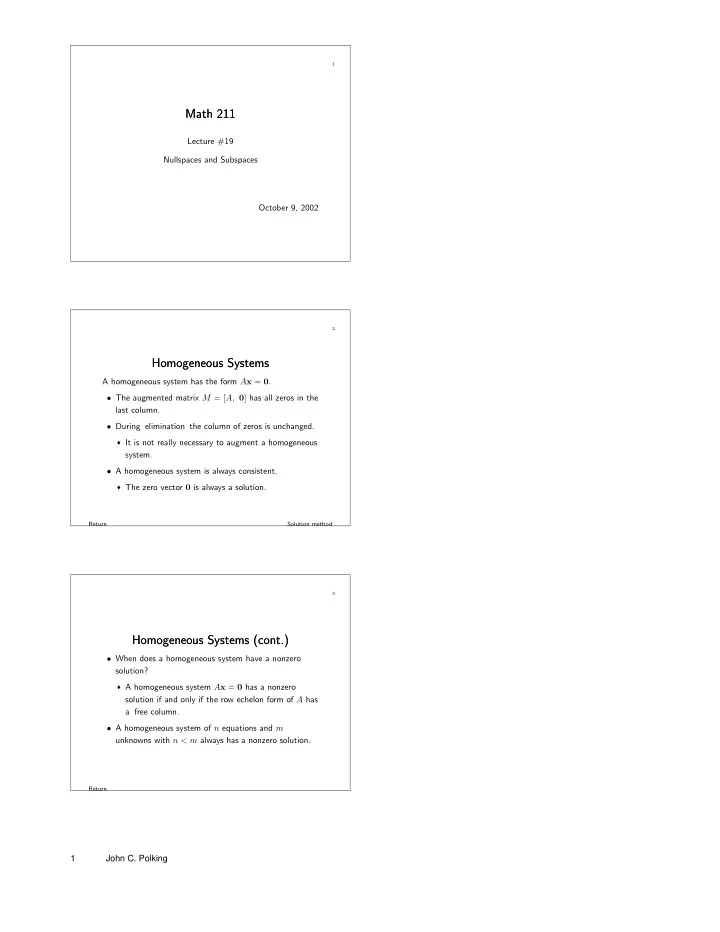
Math 211 Math 211 Lecture #19 Nullspaces and Subspaces October 9, - - PDF document

1

Math 211 Math 211

Lecture #19 Nullspaces and Subspaces October 9, 2002

Return Solution method

2

Homogeneous Systems Homogeneous Systems

A homogeneous system has the form Ax = 0.

• The augmented matrix M = [A, 0] has all zeros in the

last column.

• During elimination the column of zeros is unchanged.

It is not really necessary to augment a homogeneous

system.

• A homogeneous system is always consistent.

The zero vector 0 is always a solution.

Return

3

Homogeneous Systems (cont.) Homogeneous Systems (cont.)

• When does a homogeneous system have a nonzero

solution?

A homogeneous system Ax = 0 has a nonzero

solution if and only if the row echelon form of A has a free column.

• A homogeneous system of n equations and m

unknowns with n < m always has a nonzero solution. 1 John C. Polking

Return

4

Example 1 Example 1

A =   1 3 2 −1 4 1 1 5  

• The solution set to Ax = 0 is x = t(−3, −2, 1)T for

−∞ < t < ∞.

There are nonzero solutions because the reduced

echelon form of A has a free column.

• The system Ax = (1, 1, 0)T has no solutions.

The reduced echelon form of M = [A, b] has a pivot

in the last column.

Return Example 1

5

Example 2 Example 2

B =   1 3 2 −1 4 1 1 4  

• The reduced echelon form of B has no free columns.
• The solution set for the homogeneous system Bx = 0

has no nonzero solutions.

• The inhomogeneous system Bx = b has a unique

solution for any vector b.

Return Example 1 Example 2

6

Square Homogenous Systems Square Homogenous Systems

Suppose that A is a square (n × n) matrix.

• If the homogeneous system Ax = 0 has a nonzero

solution then there are vectors b for which the system Ax = b has no solutions.

• If the homogeneous system Ax = 0 has no nonzero

solutions then the system Ax = b has a unique solution for every vector b. 2 John C. Polking

Return Example 1 Example 2

7

Singular and Nonsingular Matrices Singular and Nonsingular Matrices

The n × n matrix A is nonsingular if the equation Ax = b has a solution for any choice of right hand side b. Proposition: The n × n matrix A is nonsingular if and

• nly if the row echelon form
• f A has only nonzero

entries along the diagonal.

• A is nonsingular ⇔ the reduced row echelon form of A

is the identity matrix I.

Return Example 1 Example 2

8

Properties of Singular and Nonsingular Matrices Properties of Singular and Nonsingular Matrices

Proposition: If the n × n matrix A is nonsingular then the equation Ax = b has a unique solution for any right hand side b. Proposition: The n × n matrix A is singular if and only if the homogeneous equation Ax = 0 has a non-zero solution.

• This is a result that we will use repeatedly.

Return

9

Invertible Matrices Invertible Matrices

An n × n matrix A is invertible if there is an n × n matrix B such that AB = BA = I. The matrix B is called an inverse of A.

• If B1 and B2 are both inverses of A, then B1 = B2.
• The inverse of A is denoted by A−1.
• Invertible ⇒ nonsingular.
• Nonsingular ⇒ invertible.

3 John C. Polking

10

Computing the inverse A−1 Computing the inverse A−1

• Form the matrix [A, I].
• Do elimination until the matrix is in reduced row

echelon form.

If A is invertible this will have the form [I, B].

• Then A−1 = B.
• Examples:

1 2 2 3

• ,

a b c d

• , B =

  1 3 2 −1 4 1 1 4  

• In MATLAB use inv.

Return

11

The Solution Set of Ax = b The Solution Set of Ax = b

• Example: The matrix A from Example 1 with

b = (7, 13, 8)T . x = (7, 1, 0)T + t(−3, −2, 1)T . Theorem: Let xp be a particular solution to Axp = b.

• 1. If Axh = 0 then x = xp + xh also satisfies Ax = b.
• 2. If Ax = b, then there is a vector xh such that

Axh = 0 and x = xp + xh.

• Thus, the solution set for Ax = b is known if we know
• ne particular solution xp and the solution set for the

homogeneous system Axh = 0.

Return Solution set

12

Solution Set of a Homogeneous System Solution Set of a Homogeneous System

• The solution set for the homogeneous system Ax = 0

is called the nullspace of the matrix A. It is denoted by null(A). Thus null(A) = {x | Ax = 0} .

• What are the properties of nullspaces?
• Is there a convenient way to describe them?

4 John C. Polking

Return

13

Properties of Nullspaces Properties of Nullspaces

Proposition: Let A be a matrix.

• 1. If x and y are in null(A), then x + y is in null(A).
• 2. If a is a scalar and x is in null(A), then ax is in

null(A). Definition: A nonempty subset V of Rn that has the properties

• 1. if x and y are vectors in V , x + y is in V ,
• 2. if a is a scalar, and x is in V , then ax is in V ,

is called a subspace of Rn.

Return

14

Examples of Subspaces Examples of Subspaces

• The nullspace of a matrix is a subspace.
• A line through 0, V = {tv | t ∈ R} , is a subspace.
• A plane through 0, V = {av + bw | a, b ∈ R} , is a

subspace.

• {0} and Rn are subspaces of Rn.

These are called the trivial subspaces.

Return

15

Linear Combinations Linear Combinations

Proposition: Any linear combination of vectors in a subspace V is also in V .

• Subspaces of Rn have the same linear structure as Rn

itself.

• The nullspace of a matrix is a subspace, so it has the

same linear structure as Rn. 5 John C. Polking

Return

16

Example Example

A =   4 3 −1 −3 −2 1 1 2 1   The nullspace of A is the set null(A) = {av | a ∈ R} , where v = (1, −1, 1)T .

Return Previous example

17

Example Example

B =   4 3 −1 6 −3 −2 1 −4 1 2 1 4   The nullspace of B is the set null(B) = {av + bw | a, b ∈ R} , where v = (1, −1, 1, 0)T and w = (0, −2, 0, 1)T .

• null(B) consists of all linear combinations of v and w.

Return null(A) null(B) Examples

18

The Span of a Set of Vectors The Span of a Set of Vectors

In every example the subspace has been the set of all linear combinations of a few vectors. Definition: The span of a set of vectors is the set of all linear combinations of those vectors. The span of the vectors v1, v2, . . . , and vk is denoted by span(v1, v2, . . . , vk). Proposition: If v1, v2, . . . , and vk are all vectors in Rn, then V = span(v1, v2, . . . , vk) is a subspace of Rn. 6 John C. Polking

Return Span

19

How do we know if w is in span(v1, v2, . . . , vk)? How do we know if w is in span(v1, v2, . . . , vk)?

1. Form the matrix V = [v1, v2, · · · .vk] which has the vectors v1, v2, . . . , and vk as its columns. 2. Solve the system V a = w. a. If there are no solutions, w is NOT in span(v1, v2, . . . , vk)? b. If there is a solution a = (a1, a2, · · · , ak)T , then w = a1v1 + a2v2 + . . . + akvk.

Return Span

20

Examples Examples

Let v1 = (1, 2)T , v2 = (1, 0)T , and v3 = (2, 0)T .

• span(v1, v2) = R2. (Proof?)
• span(v1, v3) = R2. (Proof?)
• span(v2, v3) = span(v2). (Proof?)

span(v2, v3) = {tv2 | t ∈ R} . v2 and v3 have the same direction.

Return

21

Row operations Row operations

The permissable operations on the rows of the augmented matrix are called row operations.

• Add a multiple of one row to another.
• Interchange two rows.
• Multiply a row by a non-zero number.

7 John C. Polking

Return

22

Row Echelon Form Row Echelon Form

A matrix is in row echelon form if every pivot lies strictly to the right of those in rows above.            P ∗ ∗ ∗ ∗ ∗ ∗ ∗ ∗ P ∗ ∗ ∗ ∗ ∗ ∗ ∗ P ∗ ∗ ∗ ∗ ∗ P ∗ ∗ ∗ ∗ P ∗ ∗ P ∗           

• P is a pivot, ∗ is any number.

Return

23

Method of Solution for Ax = b Method of Solution for Ax = b

The method is called elimination and backsolving, or Gaussian elimination. There are four steps: 1. Use the augmented matrix M = [A, b]. 2. Use row operations to reduce the augmented matrix to row echelon form. 3. Write down the simplified system. 4. Backsolve.

Assign arbitrary values to the free variables. Backsolve for the pivot variables.

8 John C. Polking