Math 140 of the American public assigns a grade of A or B to the - - PowerPoint PPT Presentation

SLIDE 1

1

Math 140 Introductory Statistics

Professor Silvia Fernández Chapter 8 Based on the book Statistics in Action by A. Watkins, R. Scheaffer, and G. Cobb.

8.1 Estimating a Proportion with Confidence

A recent Phi Delta Kappa/Gallup poll reported that a record 51%

• f the American public assigns a grade of A or B to the public

schools in their community and that this survey had a margin of error of 3%. Source: 2001, www.gallup.com/poll/releases/pr010823.asp.

These results are based on telephone interviews with a

randomly selected national sample of 1108 adults, 18 years and

• lder, conducted May 23–June 6, 2001.

For results based on this sample, one can say with 95 percent

confidence that the maximum error attributable to sampling and

• ther random effects is plus or minus 3 percentage points. In

addition to sampling error, question wording and practical difficulties in conducting surveys can introduce error or bias into the findings of public opinion polls.

8.1 Estimating a Proportion with Confidence

A recent Phi Delta Kappa/Gallup poll reported that a record 51%

• f the American public assigns a grade of A or B to the public

schools in their community and that this survey had a margin of error of 3%. Source: 2001, www.gallup.com/poll/releases/pr010823.asp.

The Gallup organization is disclosing that they didn’t ask all

adults in the United States, only 1108. Even so, unless there are some special difficulties such as problems with the wording of the question, they are 95% confident that the error is less than 3% either way in the percentages they report. That is, they are 95% confident that if they were to ask all adults in the United States to give a grade to the public schools, 51% ± 3%, or between 48% and 54%, would give a grade of A or B. How can the Gallup organization possibly make such a statement?

Reasonably Likely (Again)

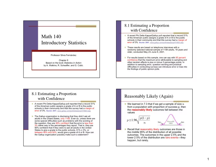
We learned in 7.3 that if we get a sample of size n

from a population with proportion of success p, then the reasonably likely outcomes fall between the values

Recall that reasonably likely outcomes are those in

the middle 95% of the distribution of all possible

• utcomes. The outcomes in the upper 2.5% and the

lower 2.5% of the distribution are rare events—they happen, but rarely.

n p p p ) 1 ( 96 . 1 − ±

SLIDE 2

2

Examples

Example p.468. Suppose that you will flip a fair coin

100 times. What are the reasonably likely values of the sample proportion ? What numbers of heads are reasonably likely?

• D1. Suppose 35% of a population think they pay too

much for car insurance. A polling organization takes a random sample of 500 people in this population and computes the sample proportion of people who think that they pay too much for car insurance.

• a. There is a 95% chance that will be between what

two values?

• b. Is it reasonably likely to get 145 people in the

sample who think they pay too much for car insurance?

p ˆ p ˆ

Activity 8.1b

• 1. Your instructor will give you
• ne of the population propor-

tions whose line segments are missing in Display 8.1.

• 2. Compute the reasonably

likely outcomes for your population proportion p.

• 3. On your copy of the chart in

Display 8.1, draw a horizontal line segment showing the reasonably likely outcomes for your group’s proportion p.

• 4. Get the reasonably likely
• utcomes from the other

groups in your class and complete the chart with the line segments from those values of

p.

Activity 8.2 Results

0.8841 0.6158 0.75 0.8420 0.5579 0.7 0.7978 0.5021 0.65 0.7518 0.4481 0.6 0.7041 0.3958 0.55 0.6549 0.3450 0.5 0.6041 0.2958 0.45 0.5518 0.2481 0.4 0.4978 0.2021 0.35 0.4420 0.1579 0.3 0.3841 0.1158 0.25 Right Left

p

Example: Plausible Percentages

In a group of 40 adults, exactly 30 were right-eye dominant.

Assuming this can be considered a random sample of all adults, is it plausible that if you tested all adults, you would find that 50% are right-eye dominant? Is it plausible that 80% are right- eye dominant? What percentages are plausible?

SLIDE 3

3

Confidence Interval

A 95% confidence interval consists of those

population percentages p for which the sample proportion p is reasonably likely.

Notes:

In the previous diagram the horizontal

segments were reasonably likely intervals.

The 95% confidence intervals should be

represented as vertical segments. In this case

p is the unknown parameter. In the previous

example the 95% confidence interval goes from 0.6 to about 0.85

. ˆ

Discussion: Confidence Intervals

• D3. According to the 2000 U.S. Census, about 60% of Hispanics

in the United States are of Mexican origin. Would it be reasonably likely in a survey of 40 randomly chosen Hispanics to find that 27 are of Mexican origin?

Source: www.census.gov/prod/2001pubs/c2kbr01

• 3

.pdf.

• D4. According to the 2000 U.S. Census, about 30% of people
• ver age 85 are men. In a random sample of 40 people over age

85, would it be reasonably likely to get 60% who are men?

Source: www.census.gov/prod/2001pubs/c2kbr01

• 1

0.pdf.

• D5. Suppose that in a random sample of 40 toddlers, 34 know

what color Elmo is. What is the 95% confidence interval for the percentage of toddlers who know what color Elmo is?

• D6. Polls usually report a margin of error. Suppose a poll of 40

randomly selected statistics majors finds that 20 are female. The poll reports that 50% of statistics majors are female, with a margin of error of 15%. Use your completed chart to explain where the 15% came from.

Getting a Formula

• The endpoints of the horizontal

segment (a reasonably likely interval) are:

• The horizontal segments are

delimited by two curves that are almost parallel lines of slope 1.

• Thus the vertical segment has

about the same length as the horizontal segment.

• Moreover, since the center of

each horizontal segment is p, then the endpoints of the vertical segment are:

n p p p ) 1 ( 96 . 1 − ± n p p p ) ˆ 1 ( ˆ 96 . 1 ˆ − ±

A Confidence Interval for a Proportion. (Any percent)

A confidence interval for the proportion of successes p in the

population is given by the formula

n is the sample size, is the proportion of successes in the sample.

The value of z depends on how confident you want to be that will be in the confidence interval. For a 95% confidence interval, use z = 1.96; for a 90% confidence interval, use z = 1.645; for a 99% confidence interval, use z = 2.576; and so on.

This confidence interval is reasonably accurate when three

conditions are met:

The sample was a simple random sample from a binomial

population (every subject is either a success or a failure).

Both The size of the population is at least 10 times the size of the

sample n.

n p p z p ) ˆ 1 ( ˆ ˆ − ⋅ ±

p ˆ 10. least at are ) ( and p n p n ˆ 1 ˆ − p ˆ

SLIDE 4

4

A Confidence Interval and the Margin of Error

• A confidence interval for the

proportion of successes p in the population is given by the formula

• This confidence interval is

reasonably accurate when three conditions are met:

The sample was a SRS

from a binomial population (every subject is either a success or a failure).

• The size of the population is

at least 10 times the size of the sample n.

n p p z p ) ˆ 1 ( ˆ ˆ − ⋅ ±

. 10 ˆ 1 10 ˆ ≥ − ≥ ) ( and p n p n ⎪ ⎩ ⎪ ⎨ ⎧ = confidence 99% for confidence 95% for confidence 90% for 576 . 2 96 . 1 645 . 1 z

n p p z E ) ˆ 1 ( ˆ − ⋅ =

• The quantity

is called the margin of error. It is half the length of the confidence interval.

Example: Safety Violations.

Suppose you have a random sample of 40

buses from a large city and find that 24 have a safety violation. Find the 90% confidence interval for the proportion of all buses that have a safety violation.

Activity 8.3 (Simulated)

• 1. Generate a random sample of

40 numbers between 0 and 9.

• 2. Count the number of even digits

in your sample of 40.

• 3. Construct a 95% confidence

interval for the proportion of random digits that are even.

• 4. Repeat a 100 times and draw all
• f the intervals in the

appropriate display (like Display 8.5 in p. 426)

• 5. What is the true proportion of all

random digits that are even?

• 6. What percentage of the

confidence intervals captured the true proportion? Is this what you expected? Explain.

• Examples:

1 6 9 6 3 0 9 1 3 1 2 8 3 5 6 0 0 0 6 7 8 3 1 4 9 6 5 6 9 6 7 5 3 2 6 8 1 4 1 2 Even: 20

• 8 9 4 4 2 6 6 8 7 4 9 6 3 4 8 8 2

7 4 4 2 0 3 6 1 6 0 5 2 0 9 8 2 7 2 1 7 2 5 8 Even: 27 ) 65495 . , 34505 . ( 40 ) 5 . 1 ( 5 . ) 96 . 1 ( 5 . Interval Confidence 95% = − ± 5 . 40 20 ˆ = = p 675 . 40 27 ˆ = = p ) 82015 . , 52985 . ( 40 ) 675 . 1 ( 675 . ) 96 . 1 ( 675 . Interval Confidence 95% = − ±

Activity 8.3 (Simulated)

• Examples:

1 6 9 6 3 0 9 1 3 1 2 8 3 5 6 0 0 0 6 7 8 3 1 4 9 6 5 6 9 6 7 5 3 2 6 8 1 4 1 2 Even: 20

• 8 9 4 4 2 6 6 8 7 4 9 6 3 4 8 8 2

7 4 4 2 0 3 6 1 6 0 5 2 0 9 8 2 7 2 1 7 2 5 8 Even: 27 ) 65495 . , 34505 . ( 40 ) 5 . 1 ( 5 . ) 96 . 1 ( 5 . Interval Confidence 95% = − ± 5 . 40 20 ˆ = = p 675 . 40 27 ˆ = = p ) 82015 . , 52985 . ( 40 ) 675 . 1 ( 675 . ) 96 . 1 ( 675 . Interval Confidence 95% = − ±

SLIDE 5

5

Activity 8.3 (Simulated)

How many intervals contain the true proportion of even numbers p = 0.5? Answer: all except one, that is 38 out of

• 39. Or 97.43% of all of the intervals.

In general, if we randomly calculate a large number of 95% Confidence Intervals we should expect that about 95% of them will contain the true value of p.

Back to Opinion Polls.

At the beginning of this section, you read about a recent Phi

Delta Kappa/Gallup poll that reported that a record 51% of the American public assigns a grade of A or B to the public schools in their community. The sample size was 1108. This survey had a margin of error of 3%, and so their 95% confidence interval is 48% to 54%. (The procedure Gallup uses to select a sample is more complicated than simple random sampling, but you can use your formula for a confidence interval to approximate Gallup’s margin of error.) You now should be able to answer these questions:

What is it that you are 95% sure is in the confidence interval?

Answer: The proportion of all Americans who would assign a grade of A or B to their local public schools.

Back to Opinion Polls.

At the beginning of this section, you read about a recent Phi

Delta Kappa/Gallup poll that reported that a record 51% of the American public assigns a grade of A or B to the public schools in their community. The sample size was 1108. This survey had a margin of error of 3%, and so their 95% confidence interval is 48% to 54%. (The procedure Gallup uses to select a sample is more complicated than simple random sampling, but you can use your formula for a confidence interval to approximate Gallup’s margin of error.) You now should be able to answer these questions:

What is the interpretation of the confidence interval of 48% to

54%? Answer: We are 95% confident that if we could ask all Americans to give a grade to their local public schools, between 48% and 54% of them would give an A or B.

Back to Opinion Polls.

At the beginning of this section, you read about a recent Phi

Delta Kappa/Gallup poll that reported that a record 51% of the American public assigns a grade of A or B to the public schools in their community. The sample size was 1108. This survey had a margin of error of 3%, and so their 95% confidence interval is 48% to 54%. (The procedure Gallup uses to select a sample is more complicated than simple random sampling, but you can use your formula for a confidence interval to approximate Gallup’s margin of error.) You now should be able to answer these questions:

What is the meaning of “95% confidence”?

Answer: If we were to take 100 random samples of Americans and compute the 95% confidence interval from each sample, then we expect that 95 of them will contain the true proportion of all Americans that would assign a grade of A or B (whatever that proportion is).

SLIDE 6

6

What sample size should you use?

• Example. (p.426) Suppose you take a survey

and get = 0.7. If your sample size is 100, what would be the margin of error for a 95% confidence interval?

If you quadruple your sample, what would be

the new margin of error?

p ˆ

n p p z E ) ˆ 1 ( ˆ − ⋅ = 0898 . 100 ) 7 . 1 ( 7 . ) 96 . 1 ( = − = n p p z E ) ˆ 1 ( ˆ − ⋅ = 0449 . 400 ) 7 . 1 ( 7 . ) 96 . 1 ( = − =

What sample size should you use?

Simple Answer: In general, the larger the sample the more

accurate the results will be (smaller margin of error). If we would like to find the sample size for a particular margin of error, all we have to do is solve for n.

n p p z E ) ˆ 1 ( ˆ − ⋅ = ⎟ ⎠ ⎞ ⎜ ⎝ ⎛ − ⋅ = n p p z E ) ˆ 1 ( ˆ

2 2 2 2

) ˆ 1 ( ˆ E p p z n − ⋅ =

If you do not have an estimate for , then you should use 0.5. You may get a larger n than you need but never a smaller one.

p ˆ

Example: Estimating needed sample sizes (p.481)

What sample size should you use for a

survey if you want the margin of error to be at most 3% with 95% confidence but you have no estimate of p?

• D17. Suppose it costs $1 to survey each

person in your sample. You judge that p is about 0.5. What will your survey cost if you want a margin of error of about 10%? 1%? 0.1%?

8.2 Testing a Proportion

People often make decisions with data by comparing

the results from a sample to some predetermined

• standard. These kinds of decisions are called tests
• f significance.

Goal: To test the significance of the difference

between the sample and the standard.

Small difference: there is no reason to conclude that

the standard doesn’t hold.

Large enough difference: If it can’t reasonably be

attributed to chance, you can conclude that the standard no longer holds.

SLIDE 7

7

Example

About 2% of barn swallows have

white feathers in places where the plumage is normally blue or red. The white feathers are caused by genetic mutations.

• In 1986, the Russian nuclear

reactor at Chernobyl leaked

• radioactivity. Researchers

continue to be concerned that the radiation may have caused mutations in the genes of humans and animals that were passed on to offspring.

Example

In a sample of barn swallows

captured around Chernobyl in 1991 and 1996, about 14% had white feathers in places where the plumage is normally blue or red.

Researchers compared the

proportion 0.14 in the sample of captured barn swallows to the standard of .02. If the overall percentage was still only 2%, it is not reasonably likely to get 14% in their sample.

So they came to the conclusion that

there was an increased probability

• f genetic mutations in the

Chernobyl area. Source: Los Angeles Times,

October 9, 1997, page B2.

Informal Significance Testing

People tend to believe that

pennies are balanced. They generally have no qualms about flipping a penny to make a fair

• decision. Is it really the case that

penny flipping is fair? What about spinning pennies?

The logic involved in deciding

whether or not to reject the standard that spinning a penny results in heads 50% of the time makes use of the same logic as that involved in estimating a proportion in Section 8.1.

Spinning Pennies Jenny and Maya’s Spins

Jenny and Maya wonder if

heads and tails are equally likely when a penny is spun. They spin pennies 40 times and get 17 heads. Should they reject the standard that pennies fall heads 50% of the time even if heads and tails are equally likely?

425 . 40 17 ˆ = = p

The value 0.425 falls in the reasonably likely interval

• btained from p = 0.5.

SLIDE 8

8

Statistical Significance

A sample is statistically significant if it is

not a reasonably likely outcome when the proposed standard is true.

Jenny and Maya’s result is not statistically

significant since their sample proportion of 0.425 falls within the reasonably likely interval

• f p = 0.5.

Spinning Pennies Miguel and Kevin’s Spins

Miguel and Kevin also spun

pennies and got 10 heads

• ut of 40 spins for a sample

proportion of 0.25. Is this a statistically significant result?

25 . 40 10 ˆ = = p

The value 0.25 falls outside the reasonably likely interval

• btained from p = 0.5.

This is a statistically significant result!

Spinning Pennies Miguel and Kevin’s Spins

Miguel and Kevin also spun

pennies and got 10 heads out

• f 40 spins for a sample

proportion of 0.25. Is this a statistically significant result?

The value 0.25 falls outside

the reasonably likely interval

• btained from p = 0.5.

Another solution

is to calculate the 95% Confidence Interval using and verify that 0.5 is not in it.

25 . 40 10 ˆ = = p 25 . ˆ = p

) 38419 . , 11581 . ( 40 ) 25 . 1 )( 25 . ( 96 . 1 25 . ) ˆ 1 ( ˆ 96 . 1 ˆ = = − ± = − ± n p p p

Basic Notation.

Population proportion of successes (Unknown in general) Sample proportion of successes (What we recorded from our sample) Hypothesized value of the population

• proportion. (The Standard)

p ˆ p p

SLIDE 9

9

Discussion: Statistical Significance

A 1997 article reported that two-thirds of teens in grades 7–12

want to study more about medical research. You wonder if this proportion still holds today and decide to test it. You take a random sample of 40 teens and find that only 23 want to study more about medical research.

Source: CNN Interactive Story Page, www.cnn.com/tech/9704/22/teentech.poll/, April 22, 1997.

• a. What is the standard (the hypothesized value, p0, of the

population proportion)?

• b. What is an alternate hypothesis?
• c. What is the sample proportion?
• d. Is the result statistically significant? That is, is there

evidence leading you to believe that the proportion today is different from the proportion in 1997?

Discussion: Statistical Significance

• a. What is the standard (the hypothesized value, p0,
• f the population proportion)?

Answer: p0 = 2/3 = 66.66%

• b. What is an alternate hypothesis?

Answer: That the proportion nowadays is different from that in 1997, that is that p0 is different from 2/3.

• c. What is the sample proportion?

Answer: The sample proportion is

575 . 40 / 23 ˆ = = p

Discussion: Statistical Significance

• d. Is the result statistically significant? That is, is

there evidence leading you to believe that the proportion today is different from the proportion in 1997?

One possible solution is to calculate the 95%

Confidence Interval and then check whether the value p0 = 2/3 is in the interval or not.

Here is the standard procedure.

Do it!

The Test Statistic

• To check if the sample proportion is statistically significant

with respect to the standard p0 we just need to check if is a rare event in the distribution generated by p0.

• We know the distribution is approximately normal with
• So we can calculate the z-score of :
• And if we get z < –1.96 or z > 1.96 then is statistically

significant.

• The numbers –1.96 and 1.96 are called critical values.

p ˆ p ˆ n p p p ) 1 ( , − = = σ μ and p ˆ p ˆ n p p p p p z ) 1 ( ˆ ˆ − − = − = σ μ This value of z is called the Test Statistic

SLIDE 10

10

Other Critical Values

• The dividing points are called critical values (denoted z*). Other z*-

values commonly used as critical points are

• If the value of the test statistic is more extreme than the critical values

you have chosen, you reject the standard and say that the result is statistically significant.

• A larger critical value makes it harder to reject the standard. If you use

z* = ±1.96, then to reject the standard, the test statistic z must fall in the

• uter 5% of the standard normal distribution. If you use z* = ±1.645, the

value of z must fall in only the outer 10% of the distribution.

• Each critical value is associated with a corresponding percentage, α

(alpha), called the level of significance. If a level of significance isn’t specified, it is usually safe to assume that α = .05 and z* = ±1.96.

1%

• f

ce significan

• f

level a for 5%

• f

ce significan

• f

level a for 10%

• f

ce significan

• f

level a for = = = α α α ⎪ ⎩ ⎪ ⎨ ⎧ = 576 . 2 96 . 1 645 . 1

*

z

Example

Find the test statistic from Jenny and Maya’s data on spinning

• pennies. (17 Heads out of 40 spins) What do you conclude if α =

0.10?

Recall that the test statistic is: Since we are testing if the probability of getting heads is 0.5,

then we have p0 = 0.5, n =40, and sample proportion p hat of 17/40 = 0.425. Thus

n p p p p z ) 1 ( ˆ − − = 948683 . 40 ) 5 . 1 ( 5 . 5 . 425 . − = − − = z

The critical values associated to α = 0.10 are z* = ±1.645. Since our test statistic falls in between, then the conclusion is that the sample is not statistically significant.

Example

Use your z-table (or your calculator preferably) to answer these

questions.

• a. What level of significance is associated with critical values
• f z* = ±2.576?

Answer: We need to find the area under the curve between – 2.576 and 2.576 in the standard normal distribution. We can do this using: normalcdf(–2.576 , 2.576)=0.9900048 So the level of significance is equal to 100% – 99% = 1%.

• b. What critical values are associated with a level of

significance of 2%? Answer: We need to find the z-values that correspond to the middle 98% of the area under the standard normal distribution, that is the values that leave 1% at the beginning and 1% at the end. By symmetry we can find only one of

• them. We can do this using:

invNorm(0.01)=–2.32634

Formal Language of Test Significance

(Components of a Significance Test for a Proportion)

• 1. Give the name of the test and check the

conditions for its use. For a significance test for a proportion, three conditions must be met.

The sample is a simple random sample from a

binomial population.

Both np0 and n(1 – p0) are at least 10. The population size is at least 10 times the sample

size.

SLIDE 11

11

Formal Language of Test Significance

(Components of a Significance Test for a Proportion)

• 2. State the hypotheses, defining any symbols.

When testing a proportion, the null hypothesis H0 is

H0 : The percentage of successes p in the population

from which the sample came is equal to p0. The alternate hypothesis, Ha, can be of three forms:

Ha : The percentage of successes p in the population

from which the sample came is not equal to p0.

Ha : The percentage of successes p in the population

from which the sample came is greater than p0.

Ha : The percentage of successes p in the population

from which the sample came is less than p0.

Formal Language of Test Significance

(Components of a Significance Test for a Proportion)

• 3. Compute the test statistic z and compare it to the

critical values z* (or find the P-value—as explained later in this section).

The test statistic is Compare the value of z to the predetermined critical

• values. Include a sketch that illustrates the situation.

n p p p p z ) 1 ( ˆ − − =

Formal Language of Test Significance

(Components of a Significance Test for a Proportion)

• 4. Write a conclusion. There are two parts to stating a

conclusion:

Say whether you reject the null hypothesis or don’t

reject the null hypothesis, linking your reason to the results of your computations.

Tell what your conclusion means in the context of the

situation. Note: You should never say that you accept the null hypothesis, because all other values in the confidence interval for p could be plausible values, you cannot assert that p0 is the right one.

Example (Similar to example on p. 499.)

• Do the whole analysis for Miguel and

Kevin’s spinning of 40 pennies getting 10 of them heads.

• That is conduct a significance test to see if a

penny comes up heads 50% of the time when spun.

SLIDE 12

12

Types of Error

There are two possible types of error in

significance testing:

Correct Type I error Reject H0 Type II error Correct Don’t Reject H0 False True Null hypothesis is actually Your decision

Type I error (When Test Statistic is Large)

If the test statistic is large in absolute value (like Miguel and

Kevin’s example), then the possible explanations for this are:

• 1. The null hypothesis is true and a rare event occurred. That

is, it was just bad luck that resulted in being so far from p0.

• 2. The null hypothesis isn’t true, and that’s why the sample

proportion was so far from p0.

• 3. The sampling process was biased in some way, and so the

sample value is itself suspicious.

If the last explanation is ruled out, then the usual decision is to

reject the null hypothesis H0. However, you may be making a Type I error—rejecting H0 even though H0 is actually true.

Type II error (When Test Statistic is Small)

If the test statistic is small in absolute value (like Jenny and

Maya’s sample), then the possible explanations for this are:

• 1. The null hypothesis is true, and you got just about what

you would expect in the sample.

• 2. The null hypothesis isn’t true, and it was just by chance

that turned out to be close to p0.

• 3. The sampling process was biased in some way, and so the

sample value is itself suspicious.

If the last explanation is ruled out, then the usual decision is to

not reject the null hypothesis H0. However, you may be making a Type II error—not rejecting H0 even though H0 is actually false.

Minimizing the Error

Type I Error. Null hypothesis is true but you reject it.

If the null hypothesis is true, then the probability of making a Type I error is equal to the significance level of the test. To decrease the probability of a Type I error, decrease the significance level. Changing the sample size has no effect

• n the probability of a Type I error.

Type II Error. Null hypothesis is false and you fail to reject

it. To decrease the probability of making a Type II error, you can take a larger sample n or you can increase the significance level α. (But if you do the last option you will increase the probability of a Type I error)

SLIDE 13

13

P-Values

Instead of just reporting that you either have or have

not rejected the null hypothesis, it has become common practice also to report a P-value.

The P-value for a test is the probability of seeing a

result from a random sample that is as extreme as or more extreme than the one you got from your random sample if the null hypothesis is true. (The P-value for a test is a conditional probability)

Example

Suppose that 22 students out of a random sample of

40 students carry a backpack to school. Follow steps a–d to test the claim that exactly half of the students in the school carry backpacks to class.

• a. Name the test and check the conditions needed for

it.

• b. State the hypotheses in words and symbols.
• c. Calculate the value of the test statistic. Calculate the

P-value for the test. Use this P-value in a sentence that explains what it represents.

• d. What is your conclusion? Explain in the context of

this problem.

One-Tailed Tests of Significance

When testing the effectiveness of a new drug, the investigator

must establish that the new drug has a better cure rate than the

• lder treatment (or that there are fewer side effects). He or she

isn’t interested in simply rejecting the null hypothesis that the new drug has the same cure rate as the older treatment. He or she needs to know if it is better. In such situations, the alternate hypothesis should state that the new drug cures a larger proportion of people than does the older treatment.

This is called a one-tailed test of significance. Tests of

significance can be one-tailed if the investigator has an indication of which way any change from the standard should

• go. This must be decided before looking at the data.

Alternate Hypothesis

• When testing a proportion, the

alternate hypothesis can take

• ne of three forms.

Ha : The percentage of

successes p in the population from which the sample came is not equal to p0.

Ha : The percentage of

successes p in the population from which the sample came is greater than p0.

Ha : The percentage of

successes p in the population from which the sample came is less than p0. Ha : p ≠ p0 Ha : p > p0 Ha : p < p0

SLIDE 14

14

Example: One-Sided Test

• f Significance

The editors of a magazine have noticed that

people seem to believe that a successful life depends on having good friends. They would like to have a story about this and use a headline such as “Most adults believe friends are important for success.” So they commissioned a survey to ask a random sample of adults whether a successful life depends on having good friends. In a random sample of 1027 adults, 53% said yes. Should the editors go ahead and use their headline?

Example: One-Sided Test

• f Significance

1. Give the name of the test and check the conditions for its use. Name: Significance test for a proportion.

n = 1027, p0 = 0.5 (the standard, if

having a succesful life is not affected by having good friends or not)

• The sample is a simple random

sample (it says in the problem), from a binomial population (a person either agrees or not that a successful life depends on good friends) .

• np0 = (1027)(0.5) = 513.5 > 10

n(1 – p0) = (1027)(1– 0.5) = 513.5 > 10

• Total number of adults

> 10 (1027) = 10270

• 2. State the hypotheses, defining

any symbols.

H0 : The proportion of

people p who believe that a successful life depends on good friends is equal to p0 = 0.5. (p = p0 )

Ha : The proportion of

people p who believe that a successful life depends on good friends is greater than p0 = 0.5 (p > p0 )

Example: One-Sided Test

• f Significance
• 3. Compute the test statistic z and find the P-value

The test statistic is And then the P-value is the probability that we get a sample with proportion greater than this test statistic (1.92) (Because we have a one-sided significance test). Thus P-value = normalcdf(1.92, 999999) = 0.0274288 92 . 1 1027 ) 5 . 1 ( 5 . 5 . 53 . = − − = z

Example: One-Sided Test

• f Significance
• 4. Write a conclusion.
• Since the P-value equals 0.0274 and this is less

than α = 0.05 = 5%. Then we should reject the null hypothesis.

• If the percentage of all adults who believe a

successful life depends on having good friends is 50% or less, then the probability of getting a sample proportion of 53% or more is only .0274. Since this value is too small this gives strong evidence that the true percentage is greater than 50%. The editors should feel free to run the headline.

SLIDE 15

15

8.3 A Confidence Interval for the Difference of two Proportions

A very common and important situation

involves taking two samples independently from two different populations with the goal of estimating the size of the difference between the proportion of successes in one population and the proportion of successes in the other.

Example

A recent poll of 29,700 U.S. households

found that 63% owned a pet. The percentage in 1994 was 56%. [Source: American Pet Products

Manufacturers Association, www.appma.org.]

The two populations are the households in

the United States in 1994 and the households

• now. The question you will investigate is:

“What was the change in the percentage of

U.S. households that own a pet?”

Intuitive Formula

A confidence interval for the difference of two

proportions, p1 − p2, where p1 is the proportion of successes in the first population and p2 is the proportion of successes in the second population: p1 and p2 are the proportions of successes in the two samples.

In our example, the 95% confidence interval for the

difference between the proportion of U.S. households that own pets now and the proportion that owned pets in 1994: b p1 b p1 b p2 b p2 ( b p1 ¡ b p2) § z¤ ¢ standard error of( b p1 ¡ b p2) ( b p1 ¡ b p2) § z¤ ¢ standard error of( b p1 ¡ b p2) (0:63 ¡ 0:56) § 1:96 ¢ standard error of( b p1 ¡ b p2) (0:63 ¡ 0:56) § 1:96 ¢ standard error of( b p1 ¡ b p2)

Standard Error of the Difference

The standard errors of the distributions of p1

and p2 can be estimated respectively as:

And if we assume the proportion samples are

independent, then the standard error of the difference can be approximated as

s b p1(1 ¡ b p1) n1 and s b p2(1 ¡ b p2) n2 s b p1(1 ¡ b p1) n1 and s b p2(1 ¡ b p2) n2

b p1 b p1 b p2 b p2

s b p1(1 ¡ b p1) n1 + b p2(1 ¡ b p2) n2 s b p1(1 ¡ b p1) n1 + b p2(1 ¡ b p2) n2

SLIDE 16

16

The Formula

The confidence interval for the difference,

p1 − p2 , of the proportion of successes in one population and the proportion of successes in the second population is,

Where p1 is the proportion of successes in a random

sample of size n1 taken from the first population, and p2 is the proportion of successes in a random sample

• f size n2 taken from the second population. (Sample

sizes do not need to be equal.) b p1 b p1 b p2 b p2 ( b p1 ¡ b p2) § z¤ ¢ s b p1(1 ¡ b p1) n1 + b p2(1 ¡ b p2) n2 ( b p1 ¡ b p2) § z¤ ¢ s b p1(1 ¡ b p1) n1 + b p2(1 ¡ b p2) n2

Conditions for use

The conditions that must be met in order to

use this formula are that

the two samples are taken randomly and

independently from two populations.

each population is at least 10 times as large

as its sample size.

n1p1, n1(1−p1), n2p2, and n2(1−p2) are all

at least 5.

b b b b b b b

Example: A Difference in Pet Ownership?

A recent pet ownership survey found that

63% of the 29,700 U.S. households sampled

• wn a pet. A 1994 survey, taken by the same
• rganization, found that 56% of the 6,786

U.S. households sampled owned a pet. Find and interpret a 95% confidence interval for the difference between the proportion of U.S. households that own a pet now and the proportion of U.S. households that owned a pet in 1994.

8.4/8.5 Significance Test for the Difference of two Proportions

Often times we need to decide which is the

greater of two proportions, or whether we can assume they are the same. For example.

Is snowboarding or skiing more likely to result

in a serious injury?

Does a new treatment for AIDS result in fewer

deaths than an old treatment?

Is Reggie Jackson’s World Series record so

much better than his play during the regular season that the difference can’t reasonably be attributed to chance?

SLIDE 17

17

Example: Two AIDS treatments

Consider a clinical trial experiment comparing two treatments for

AIDS-related complex (ARC). The investigators want to find out if there is a significant difference on the survival rates of patients who had already developed AIDS. They have two treatments, patients who were given AZT and patients who were given AZT + ACV. Here’s the data 62 49 13 AZT + ACV 90 41 Yes 131 69 Total 41 28 No Total AZT Treated with Survived?

Notation:Proportions, Sample Proportions, and Sample Sizes.

sample size of patients treated with AZT sample size of patients treated with AZT+ACV proportion of patients in the sample treated with AZT that survived proportion of patients in the sample treated with AZT+ACV that survived True proportion of survival if all patients were treated with AZT (unknown) True proportion of survival if all patients were treated with AZT+ACV (unknown)

62 49 2

ˆ = p 69

1 =

n 62

2 =

n

69 41 1

ˆ = p

2 1

p p

Assumptions about the difference of two proportions.

If we have obtain two independent sample proportions

p and p , then the distribution of the difference of the two proportions p1-p2 is approximately normal as long as each proportion satisfies the following three conditions:

Each sample p and p is a simple random sample from a

binomial population, and they are independent from each other.

• r, in case of experiments, subjects were randomly assigned to

their treatments.

All the numbers n1p1, n1p2, n1(1 – p1), and n

are at least 5.

Each of the two population sizes is at least 10 times the sample

size.

1

ˆ p

2

ˆ p

2 1

ˆ ˆ p p

− 1

ˆ p

2

ˆ p ) ˆ 1 ( ), ˆ 1 ( , ˆ , ˆ

2 2 1 1 2 2 1 1

p n p n p n p n − −

Checking the conditions

Check the conditions.

We assume that subjects were randomly assigned to

treatments.

All of the following are greater than 5 The population size of AIDS patients that could

potentially be treated with AZT is clearly greater than 10 times 69 = 690 The population size of AIDS patients that could potentially be treated with AZT+ACV is clearly greater than 10 times 62 = 620

13 ) 62 / 49 1 ( 62 ) ˆ 1 ( 28 ) 69 / 41 1 ( 69 ) ˆ 1 ( 49 ) 62 / 49 ( 62 ˆ , 41 ) 69 / 41 ( 69 ˆ

2 2 1 1 2 2 1 1

= − = − = − = − = = = = p n p n p n p n

SLIDE 18

18

Writing the hypothesis

The null hypothesis

H0 : The new therapy (AZ+ACV) is as good as the old

therapy (AZT). That is the survival rate if all patients were treated with AZT+ACV would be equal to the survival rate if all patients were treated with AZT. In symbols The alternate hypothesis

Ha : The new therapy (AZ+ACV) is better than the old

therapy (AZT). That is the survival rate if all patients were treated with AZT+ACV would be greater than the survival rate if all patients were treated with AZT. In symbols

2 1 2 1

= =

− p

p p p

• r

2 1 2 1

< <

− p

p p p

• r

The Test Statistic

The test statistic in general

follows the form

The parameter is p1 – p2,

and if the null hypothesis is true then p1 – p2 = 0.

The estimate is what we

• btain for the difference of

the two proportions according to our samples.

Now, the standard deviation of

the estimate under the assumption that p1 = p2 can be approximated by

Where p is the pooled estimate

estimate

• f

deviation standard parameter estimate Statistic Test − =

196 . 790 . 594 . ˆ ˆ

2 1

− = − = =

−

estimate p p ⎟ ⎟ ⎠ ⎞ ⎜ ⎜ ⎝ ⎛ +

− 2 1

1 1 ) ˆ 1 ( ˆ n n p p 687 . 131 90 ˆ ≈ = = total grand survived total p p ˆ

The Test Statistic

The parameter is p1 – p2 = 0, The standard deviation of

the estimate

p is the pooled estimate so the standard deviation of the

estimate is:

and the test statistic:

estimate

• f

deviation standard parameter estimate Statistic Test − =

196 . 790 . 594 . ˆ ˆ

2 1

− = − = =

−

estimate p p ⎟ ⎟ ⎠ ⎞ ⎜ ⎜ ⎝ ⎛ +

− 2 1

1 1 ) ˆ 1 ( ˆ n n p p 687 . 131 90 ˆ ≈ = = total grand survived total p p ˆ 081145 . 62 1 69 1 ) 687 . 1 )( 687 . ( = ⎟ ⎠ ⎞ ⎜ ⎝ ⎛ +

−

415429 . 2 081145 . 196 . − = − −

P-Value

To get the P-Value we use the fact that the

distribution of the difference is approximately normal.

Since our test is one-sided we need to calculate the

probability that the difference is less than our test- statistic.

We can find P by doing

normalcdf(– 999999,– 2.4154)=.007858

SLIDE 19

19

Conclusion

Since the P-Value equals 0.78% and this is

definitely less than 5% we reject the null hypothesis.

If both treatments were equally effective (null

hypothesis is true) then there is only a 0.78% chance of getting a difference p1-p2 as small or smaller than – 0.196. This probability is so small that we are confident that if all subjects in the experiment had been given AZT+ACV there would be a larger survival rate than if they had received only AZT.

2 1

ˆ ˆ p p

−

Components of a Significance Test for the Difference of two Proportions

See pages 531-532 in your book.

Example E65 (page 537)

A poll of 256 boys and 257 girls age 12 to 17 asked, “Do you

feel like you are personally making a positive difference in your community?” More girls (195) than boys (161) answered “yes.”

• a. Using a one-sided test, is this a statistically significant

difference? That is, if all teens were asked, are you confident that a larger proportion of girls than boys would say “yes”? Assume that the samples were selected randomly.

• b. The report says, “Participants were selected through

random digit dialing.” Do you have any concerns about whether such a procedure would give a random sample?

• c. Find a 95% confidence interval for the proportion of all

teens who would answer yes. What additional assumption do you need to make to do this?