Markov Decision Processes (MDPs) and Reinforcement Learning (RL) - - PDF document

12/18/2019 1

Markov Decision Processes (MDPs) and Reinforcement Learning (RL)

Sven Koenig, USC

Russell and Norvig, 3rd Edition, Sections 17.1-17.2 These slides are new and can contain mistakes and typos. Please report them to Sven (skoenig@usc.edu).

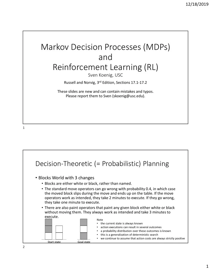
Decision-Theoretic (= Probabilistic) Planning

• Blocks World with 3 changes
• Blocks are either white or black, rather than named.
• The standard move operators can go wrong with probability 0.4, in which case

the moved block slips during the move and ends up on the table. If the move

• perators work as intended, they take 2 minutes to execute. If they go wrong,

they take one minute to execute.

• There are also paint operators that paint any given block either white or black

without moving them. They always work as intended and take 3 minutes to execute.

Start state Goal state Note

• the current state is always known
• action executions can result in several outcomes
• a probability distribution over these outcomes is known
• this is a generalization of deterministic search
• we continue to assume that action costs are always strictly positive

1 2

12/18/2019 2

Evaluating Decision-Theoretic Plans

expected plan-execution cost (here: time) 6 minutes start state goal state probability/cost = 1.0/3 1.0/3 start state goal state 0.6/2 1.0/3 0.4/1 0.6/2 0.4/1 expected plan-execution cost c1 = 5.67 minutes

Evaluating Decision-Theoretic Plans

• We assume that the expected operator cost and the probability

distribution over the successor states depend only on the current state and the operator executed in it (“Markov property”). In other words, it does not matter how the current state was reached.

• An example that illustrates the resulting independence assumptions:
• p(st+2=s’’|at+1=a’,at=a,st=s)

= Σs’ p(st+2=s’’,st+1=s’|at+1=a’,at=a,st=s) = Σs’ p(st+2=s’’ | at+1=a’,st+1=s’,at=a,st=s) p(st+1=s’|at+1=a’,at=a,st=s) = Σs’ p(st+2=s’’ | at+1=a’,st+1=s’) p(st+1=s’|at=a,st=s)

This is similar to deterministic search, where we assume that the

• perator cost and the successor state depend only on the current

state and the operator executed in it.

3 4

12/18/2019 3

Evaluating Decision-Theoretic Plans

• ci = expected plan-execution cost until a goal

state is reached if one starts in state si and follows the plan

• c1 = 0.4 (1+c2) + 0.6 (2+c3)

c2 = 0.4 (1+c2) + 0.6 (2+c3) c3 = 1.0 (3+c4) c4 = 0

• c1 = c2 = 5.67

c3 = 3 c4 = 0

start state goal state 1.0/3 0.4/1 0.6/2 0.4/1 s1 s3 s2 s4 p(st+1=s3|st=s1,at=move C to D)=0.6 / c(s1,move C to D,s3)=2 0.6/2

Evaluating Decision-Theoretic Plans

• In general, one solves the following system of equations calculating

the expected plan-execution cost of decision-theoretic plans:

• ci = 0

if si is a goal state

• ci = Σk p(sk|si,a(si)) (c(si,a(si),sk) + ck)

if si is not a goal state

• One solves the system of equations either with Gaussian elimination

(as on the previous slide) or as follows:

• for all i
• ci,0 = 0
• for t=0 to ꝏ
• for all i
• ci,t+1 = 0

if si is a goal state

• ci,t+1 = Σk p(sk|si,a(si)) (c(si,a(si),sk) + ck,t)

if si is not a goal state The typical termination criterion is: |ci,t+1 – ci,t| < ε for all i (for a given small positive ε). Later, we will call this the q-value qt+1(si,a(si)).

5 6

12/18/2019 4

Decision-Theoretic Planning Decision-Theoretic Planning

• Assumption: One has to execute operators forever

if one does not reach a goal state earlier.

• The resulting decision tree is infinite. Thus, one

cannot start at the chance nodes and propagate the values toward the root of the decision tree.

This is similar to deterministic search.

7 8

12/18/2019 5

Decision-Theoretic Planning

The optimal actions associated with these choice nodes are identical since the subtrees rooted in the choice nodes are identical. Thus, whenever the state (= configuration of blocks) is the same, one can execute the same operator. A mapping from states to operators is called “policy.” One only needs to consider all policies to determine a plan with minimal expected plan-execution cost.

This is similar to deterministic search, where one only needs to consider all paths without cycles from the start state to a goal state to determine a plan with minimal plan-execution cost.

Decision-Theoretic Planning

• This is, for example, a policy although policies are typically written as

functions that map each state to the action that should be executed in it.

start state goal state 0.6/2 1.0/3 0.4/1 0.6/2 0.4/1

9 10

12/18/2019 6

Decision-Theoretic Planning

• In the deterministic case:
• Out of all possible plans, we need to consider only cycle-free paths because

there is always a cycle-free path that is cost-minimal. This insight dramatically reduces the number of plans that we need to consider. However, it still takes too long to consider all cycle-free paths and determine one of minimal cost. Thus, we needed to study more sophisticated search algorithms.

• In the probabilistic case:
• Out of all possible plans, we need to consider only policies because there is

always a policy that is cost-minimal. This insight dramatically reduces the number of plans that we need to consider. However, it still takes too long to consider all policies and determine one of minimal expected cost. Thus, we now study more sophisticated search algorithms (here: stochastic dynamic programming algorithms).

Decision-Theoretic Planning

• We now study the case where we have a model available, that is,

know all actions and their effects. This model is specified as an MDP (Markov Decision Process). We use this model for planning.

11 12

12/18/2019 7

MDP Notation

This is similar to a state space in the context of deterministic searches. 0.4/1 0.6/2 1.0/1 0.5/1 0.5/3 = p(s3|s2,o4)/c(s2,o4,s3) 0.3/4 0.7/1

• 1
• 2
• 3
• 4

goal state

s1 s2 s3

• We do not need to label the start state since we will find a policy with

minimal expected plan-execution cost from any state to the goal state.

• The stop operator is automatically assigned to all goal states (here: s3).
• 5

1.0/5

MDP Planning

• We have a chicken-and-egg problem:
• If one knows the optimal actions (o2 in s1, o4 in s2 and stop in s3), one can

calculate the expected goal distances as shown earlier:

• c1 = 0.7 (1+c2) + 0.3 (4+c3) (= 5.08)

c2 = 0.5 (1+c1) + 0.5 (3+c3) (= 4.54) c3 = 0

Different from deterministic search, the policy with minimal expected plan-execution cost can have cycles, which complicates planning.

13 14

12/18/2019 8

MDP Planning

• We have a chicken-and-egg problem:
• If one knows the expected goal distances (c1=5.08 for s1, c2=4.54 for s2 and

c3=0.00 for s3), one can calculate the optimal actions by greedily assigning the action to each state that decreases the expected goal distance the most:

• If one executes o1 [o2] in s1 and uses the given expected goal distances as expected

minimal costs to get from the resulting successor state to a goal state, then the total expected cost to get from s1 to a goal state is 0.4 (1+c1) + 0.6 (2+c2) = 6.36 [0.7 (1+c2) + 0.3 (4+c3) = 5.08]. Since min(6.36,5.08) = 5.08, one should execute o2 in s1.

• If one executes o3 [o4] in s2 and uses the given expected goal distances as expected

minimal costs to get from the resulting successor state to a goal state, then the total expected cost to get from s2 to a goal state is 1.0 (1+c1) = 6.08 [0.5 (1+c1) + 0.5 (3+c3) = 4.54]. Since min(6.08,4.54) = 4.54, one should execute o4 in s2.

• One should stop in s3 since s3 is a goal state.

Different from deterministic search, the policy with minimal expected plan-execution cost can have cycles, which complicates planning.

MDP Planning

• Unfortunately, one neither knows the optimal actions nor the

expected goal distances. Thus, one needs to calculate them

• simultaneously. We present two methods for doing that, namely

value iteration and policy iteration.

15 16

12/18/2019 9

MDP Planning – Value Iteration

• In general, one solves the following system of equations for

calculating the expected plan-execution cost of policies:

• ci = 0

if si is a goal state

• ci = Σk p(sk|si,a(si)) (c(si,a(si),sk) + ck)

if si is not a goal state

• In general, one solves the following system of equations EQ for

finding a policy with minimal expected plan-execution cost (ci is the expected goal distance of state si):

• ci = 0

if si is a goal state

• ci = mina executable in si Σk p(sk|si,a) (c(si,a,sk) + ck)

if si is not a goal state

Called Bellman equations after an ex-faculty member at USC!

MDP Planning – Value Iteration

• One solves the system of equations EQ as follows with value iteration:
• for all i
• ci,0 = 0
• for t=0 to ꝏ
• for all i
• ci,t+1 = 0

if si is a goal state

• ci,t+1 = mina executable in si Σk p(sk|si,a) (c(si,a,sk) + ck,t)

if si is not a goal state The typical termination criterion is: |ci,t+1 – ci,t| < ε for all i (for a given small positive ε). qt+1(si,a) Improve values ci,t to values ci,t+1 by calculating the actions Pick values ci,0

17 18

12/18/2019 10

MDP Planning – Value Iteration

• It holds that ci = limt→ꝏci,t for all i.
• If one is currently in state si and can stop after executing exactly t
• perators (if one does not reach a goal state earlier), then one should

execute operator stop if si is a goal state or t=0 and operator argmina executable in si Σk p(sk|si,a) (c(si,a,sk) + ck,t)

• therwise.
• If one is currently in state si and has to execute operators forever (if
• ne does not reach a goal state earlier), then one should

execute operator stop if si is a goal state and operator argmina executable in si Σk p(sk|si,a) (c(si,a,sk) + ck)

• therwise.

MDP Planning – Value Iteration

0.4/1 0.6/2 1.0/1 0.5/1 0.5/3 = p(s3|s2,o4)/c(s2,o4,s3) 0.3/4 0.7/1

• 1
• 2
• 3
• 4

goal state

s1 s2 s3

• 5

1.0/5

19 20

12/18/2019 11

MDP Planning – Value Iteration

cs1,iteration cs2,iteration cs3,iteration

MDP Planning – Value Iteration

• If one can stop after executing exactly 3 operators, then
• first operator execution: execute o2 in s1, o4 in s2 and stop in s3 (see iteration 3)
• second operator execution: execute o2 in s1, o3 in s2 and stop in s3 (see iteration 2)
• third operator execution: execute o1 in s1, o3 in s2 and stop in s3 (see iteration 1)
• This is not a policy! (The start state does not matter.)

cs1,iteration cs2,iteration cs3,iteration

21 22

12/18/2019 12

MDP Planning – Value Iteration

• If one has to execute operators forever, then
• always: execute o2 in s1, o4 in s2 and stop in s3 (see iteration 9999)
• This is a policy! (The start state does not matter.)

cs1,iteration cs2,iteration cs3,iteration

MDP Planning – Policy Iteration

• One solves the system of equations EQ as follows with policy iteration:
• for all i
• Pick an a0(si) from all actions executable in siso that a goal state can be reached from every state with

positive probability

• for n=0 to ꝏ
• for all i
• cn,i,0 = 0
• for t=0 to ꝏ
• for all i
• cn,i,t+1 = 0

if si is a goal state

• cn,i,t+1 = mina executable in si Σk p(sk|si,an(si)) (c(si,an(si),sk) + cn,k,t) if si is not a goal state
• for all i
• cn,i = limt→ꝏcn,i,t
• for all i
• an+1(si) = stop

if si is a goal state

• an+1(si) = argmina executable in si Σk p(sk|si,a) (c(si,a,sk) + cn,k)

if si is not a goal state The typical termination criterion is: |cn,i,t+1 – cn,i,t| < ε for all i (for a given small positive ε). qt+1(si,an(si)) The typical termination criterion is: an+1(si) = an(si) for all i. Use an+1(si) = an(si) if an(si) is still optimal. Evaluate policy an(si) by calculating the ci Improve policy an(si) to policy an+1(si) Pick policy a0(si)

23 24

12/18/2019 13

MDP Planning – Policy Iteration

• If one is currently in state si and has to execute operators forever (if
• ne does not reach a goal state earlier), then one should

execute operator an(si) in state si, where n is the largest iteration.

MDP Planning – Policy Iteration

0.4/1 0.6/2 1.0/1 0.5/1 0.5/3 = p(s3|s2,o4)/c(s2,o4,s3) 0.3/4 0.7/1

• 1
• 2
• 3
• 4

goal state

s1 s2 s3

• 5

1.0/5

25 26

12/18/2019 14

MDP Planning – Policy Iteration

aiteration(s2) aiteration(s3) aiteration(s1)

MDP Planning – Policy Iteration

aiteration(s2) aiteration(s3) aiteration(s1)

• If one has to execute operators forever, then
• always: execute o2 in s1, o4 in s2 and stop in s3 (see iteration 1)
• This is a policy! (The start state does not matter.)

27 28

12/18/2019 15

MDP Planning with Discounting

• What if there is no goal state, i.e. one has to execute operators

forever?

• Every policy now has expected plan-execution cost infinity,

i.e. looks equally good.

• Infinite plan-execution costs cause problems, since it is preferable to

incur, say, the infinite sequence of operator costs, 1 1 1 1 1 1 … than 5 5 5 5 5 5 …!

0.4/1 0.6/2 1.0/1 0.5/1 0.5/3 = p(s3|s2,o4)/c(s2,o4,s3) 0.3/4 0.7/1

• 1
• 2
• 3
• 4

s1 s2 s3

• 5

1.0/5

MDP Planning with Discounting

• One needs to change the planning objective, e.g. to
• minimizing the expected plan execution cost per operator execution or
• minimizing the expected discounted plan execution cost.
• Minimizing the expected discounted plan execution cost is a bit

simpler, so we will do that in the following.

• Everything that we do in the following can be (and is) also done if

there are goal states even though it is not necessary.

29 30

12/18/2019 16

MDP Planning with Discounting

Source: Forbes, September 15, 2011 …

MDP Planning with Discounting

• A similar example with fewer payouts (to better fit on the slide):

Jan 1, 2012 Jan 1, 2013 Jan 1, 2014 Jan 1, 2015 $25,000 $25,000 $25,000 $25,000

31 32

12/18/2019 17

MDP Planning with Discounting

• If we put $1 into a savings account with interest rate p%,

then we have $(1 + p/100) in the savings account after one year.

• We call 0 < 100/(100+p) ≤ 1 the discount factor γ (gamma).

Jan 1, 2012 Jan 1, 2013 $1 $(1 + p/100)

· (100+p)/100 · 100/(100+p)

MDP Planning with Discounting

• A similar example with fewer payouts (to better fit on the slide):
• So, for an interest rate of 5% (i.e. a discount factor of γ≈0.952),

providing an annuity of 4 payments of $25,000 each year and a lumpsum payoff of (1+ γ+ γ2+γ3) $25,000 ≈ $93,081.20 (called the total discounted cost of the annuity) are equally preferable.

Jan 1, 2012 Jan 1, 2013 Jan 1, 2014 Jan 1, 2015 $25,000 $25,000 $25,000 $25,000 + γ $25,000 (1+γ) $25,000

· γ

+ γ (1+γ) $25,000 (1+ γ+ γ2) $25,000 + γ (1+ γ+ γ2) $25,000 (1+ γ+ γ2+γ3) $25,000

· γ · γ

33 34

12/18/2019 18

MDP Planning with Discounting

• Assume that the discount factor γ is 0.95 and one wants to minimize

the expected discounted plan-execution cost.

• The infinite sequence of operator costs 1 1 1 1 1 … has a finite(!)

discounted plan-execution cost of (1+γ+γ2+…) 1 = 1/(1-γ) 1 = 20.

• The infinite sequence of operator costs 5 5 5 5 5 … has a finite(!)

discounted plan-execution cost of (1+γ+γ2+…) 5 = 1/(1-γ) 5 = 100.

• So, one now prefers the infinite sequence of operator costs 1 1 1 1 1

… over the infinite sequence of operator costs 5 5 5 5 5 …!

MDP Planning with Discounting

• A similar example with fewer payouts (to better fit on the slide):

Jan 1, 2012 $25,000 + γ (1+ γ+ γ2) $25,000 (1+ γ+ γ2+γ3) $25,000 cost at time 2012 (t) + γ expected discounted plan-execution cost at time 2013 (t+1) [from time 2013 on] expected discounted plan-execution cost at time 2012 (t) [from time 2012 on]

Earlier, we used

cost at time 2012 (t) + expected plan-execution cost at time 2013 (t+1) [from time 2013 on] expected plan-execution cost at time 2012 (t) [from time 2012 on]

35 36

12/18/2019 19

MDP Planning with Discounting – Value Iteration

• In general, one solves the following system of equations for

calculating the expected discounted plan-execution cost of policies:

• ci = 0

if si is a goal state

• ci = Σk p(sk|si,a(si)) (c(si,a(si),sk) + γ ck)

if si is not a goal state

• In general, one solves the following system of equations EQ’ for

finding a policy with minimal expected discounted plan-execution cost (ci is the expected goal distance of state si):

• ci = 0

if si is a goal state

• ci = mina executable in si Σk p(sk|si,a) (c(si,a,sk) + γ ck)

if si is not a goal state

MDP Planning with Discounting – Value Iteration

• One solves the system of equations EQ’ as follows with value iteration:
• for all i
• ci,0 = 0
• for t=0 to ꝏ
• for all i
• ci,t+1 = 0

if si is a goal state

• ci,t+1 = mina executable in si Σk p(sk|si,a) (c(si,a,sk) + γ ck,t)

if si is not a goal state the typical termination criterion is: |ci,t+1 – ci,t| < ε for all i (for a given small positive ε) qt+1(si,a) Improve values ci,t to values ci,t+1 by calculating the actions Pick values ci,0

37 38

12/18/2019 20

MDP Planning with Discounting – Value Iteration

• It holds that ci = limt→ꝏci,t for all i.
• If one is currently in state si and can stop after executing exactly t
• perators, then one should execute operator stop if si is a goal state
• r t=0 and operator

argmina executable in si Σk p(sk|si,a) (c(si,a,sk) + γ ck,t)

• therwise.
• If one is currently in state si and has to execute operators forever,

then one should execute operator stop if si is a goal state and

• perator

argmina executable in si Σk p(sk|si,a) (c(si,a,sk) + γ ck)

• therwise.

MDP Planning with Discounting – Value Iteration

• The policy with minimal expected discounted plan-execution cost depends
• n the discount factor.
• The discount factor cannot be 1 since this corresponds to finding a policy

with minimal expected plan-execution cost but, ideally, it should be close to 1 (e.g. 0.95 or 0.99).

• The smaller it is, the higher one weighs costs incurred in the immediate

future over costs incurred in the distance future.

• The discount factor can also be interpreted as the probability of not dying.
• If the interest rate is (1-γ)/γ,

then the value of receiving x dollars in a year is γ x dollars right now.

• If I die later this year with probability 1-γ and can thus no longer receive future

payoffs, then the expected value of receiving x dollars in a year is γ x dollars right now.

39 40

12/18/2019 21

MDP Planning with Discounting – Policy Iteration

• One solves the system of equations EQ’ as follows with policy iteration:
• for all i
• Pick an a0(si) from all actions executable in siso that a goal state can be reached from every state with

positive probability

• for n=0 to ꝏ
• for all i
• cn,i,0 = 0
• for t=0 to ꝏ
• for all i
• cn,i,t+1 = 0

if si is a goal state

• cn,i,t+1 = Σk p(sk|si,an(si)) (c(si,an(si),sk) + γ cn,k,t)

if si is not a goal state

• for all i
• cn,i = limt→ꝏcn,i,t
• for all i
• an+1(si) = stop

if si is a goal state

• an+1(si) = argmina executable in si Σk p(sk|si,a) (c(si,a,sk) + γ cn,k)

if si is not a goal state The typical termination criterion is: |cn,i,t+1 – cn,i,t| < ε for all i (for a given small positive ε). qt+1(si,an(si)) The typical termination criterion is: an+1(si) = an(si) for all i. Use an+1(si) = an(si) if an(si) is still optimal. Evaluate policy an(si) by calculating the ci Improve policy an(si) to policy an+1(si) Pick policy a0(si)

MDP Planning with Discounting – Policy Iteration

• If one is currently in state si and has to execute operators forever (if
• ne does not reach a goal state earlier), then one should

execute operator an(si) in state si, where n is the largest iteration.

41 42

12/18/2019 22

Decision-Theoretic Planning

• We now study the case where we do not have a model available, that

is, do not know all actions and their effects. We only know which state the agent is currently in and which actions it has available. We thus cannot plan but we can still use reinforcement learning (RL) to learn which action the agent should choose in its current state.

RL with Discounting – Q Learning

• The agent executes
• for all states s and actions a
• q(s,a) = 0
• s = start state of the agent
• repeat
• a =
• execute a and observe the resulting action cost c and successor state s’
• q(s,a) = q(s,a) + α (c + γ mina’ executable in s’ q(s’,a’) – q(s,a))
• s = s’
• until s is a goal state

random action executable in s with probability ε argmina executable in s q(s,a) with probability 1-ε If s=si, then this is an estimate of ci

43 44

12/18/2019 23

RL with Discounting – Q Learning

• The agent executes
• for all states s and actions a
• q(s,a) = 0
• s = start state of the agent
• repeat
• a =
• execute a and observe the resulting action cost c and successor state s’
• q(s,a) = q(s,a) + α (c + γ mina’ executable in s’ q(s’,a’) – q(s,a))
• s = s’
• until s is a goal state

random action executable in s with probability ε argmina executable in s q(s,a) with probability 1-ε From time to time, the agent needs to execute seemingly suboptimal actions to explore the executable actions and potentially discover actions that are better than the currently seemingly best action. Thus, it needs an exploration policy. The one used here is called ε-greedy. Exploration (here: execute a random action) Exploitation (execute the seemingly best action) If s=si, then this is an estimate of ci This should look familiar from gradient descent.

RL with Discounting – Q Learning

• Q(s,a) is called the q-value of action a in state s. It is an estimate of

the total expected discounted plan execution cost when executing action a in state s and then executing the optimal actions (until a goal state is reached, if there is one). The agent should thus always execute the action in its current state with the smallest q-value.

• RL often uses rewards instead of costs, where a reward is just a

negative cost. In this case, Q learning needs to maximize instead of minimize.

• The learning rate 0 < α is often close to zero, the exploration

probability 0 < ε is often close to zero, and the discount factor 0 < γ < 1 is often close to one.

45 46