Outline Md Md Markov Markov Decision Decision Processes - - PDF document

SLIDE 1

3/25/2017 1

Md

Markov Decision Processes

Markov Decision Processes

CSE 415: Introduction to Artificial Intelligence University of Washington Spring 2017

Presented by S. Tanimoto, University of Washington, based on material by Dan Klein and Pieter Abbeel -

• University of California.

Md

Markov Decision Processes

Outline

• Grid World Example
• MDP definition
• Optimal Policies
• Auto Racing Example
• Utilities of Sequences
• Bellman Updates
• Value Iterations

2

Md

Markov Decision Processes

Non-Deterministic Search

3

Md

Markov Decision Processes

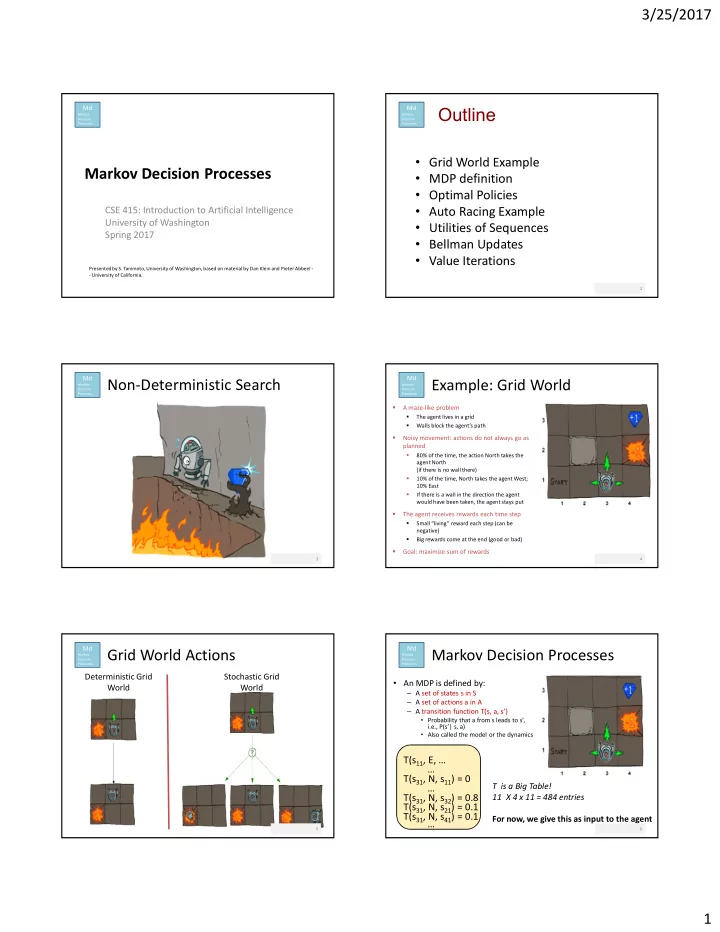
Example: Grid World

• A maze-like problem
• The agent lives in a grid
• Walls block the agent’s path
• Noisy movement: actions do not always go as

planned

• 80% of the time, the action North takes the

agent North (if there is no wall there)

• 10% of the time, North takes the agent West;

10% East

• If there is a wall in the direction the agent

would have been taken, the agent stays put

• The agent receives rewards each time step
• Small “living” reward each step (can be

negative)

• Big rewards come at the end (good or bad)
• Goal: maximize sum of rewards

4

Md

Markov Decision Processes

Grid World Actions

Deterministic Grid World Stochastic Grid World

5

Md

Markov Decision Processes

Markov Decision Processes

• An MDP is defined by:

– A set of states s in S – A set of actions a in A – A transition function T(s, a, s’)

• Probability that a from s leads to s’,

i.e., P(s’| s, a)

• Also called the model or the dynamics

T(s11, E, … … T(s31, N, s11) = 0 … T(s31, N, s32) = 0.8 T(s31, N, s21) = 0.1 T(s31, N, s41) = 0.1 …

T is a Big Table! 11 X 4 x 11 = 484 entries For now, we give this as input to the agent

6

SLIDE 2

3/25/2017 2

Md

Markov Decision Processes

Markov Decision Processes

• An MDP is defined by:

– A set of states s in S – A set of actions a in A – A transition function T(s, a, s’)

• Probability that a from s leads to s’,

i.e., P(s’| s, a)

• Also called the model or the dynamics

– A reward function R(s, a, s’)

… R(s32, N, s33) = -0.01 … R(s32, N, s42) = -1.01 R(s33, E, s43) = 0.99 …

Cost of breathing R is also a Big Table! For now, we also give this to the agent

7

Md

Markov Decision Processes

Markov Decision Processes

• An MDP is defined by:

– A set of states s in S – A set of actions a in A – A transition function T(s, a, s’)

• Probability that a from s leads to s’,

i.e., P(s’| s, a)

• Also called the model or the dynamics

– A reward function R(s, a, s’)

• Sometimes just R(s) or R(s’)

… R(s33) = -0.01 R(s42) = -1.01 R(s43) = 0.99

8

Md

Markov Decision Processes

Markov Decision Processes

• An MDP is defined by:

– A set of states s in S – A set of actions a in A – A transition function T(s, a, s’)

• Probability that a from s leads to s’, i.e.,

P(s’| s, a)

• Also called the model or the dynamics

– A reward function R(s, a, s’)

• Sometimes just R(s) or R(s’)

– A start state – Maybe a terminal state

• MDPs are non-deterministic search

problems

– One way to solve them is with expectimax search – We’ll have a new tool soon

9

Md

Markov Decision Processes

What is Markov about MDPs?

• “Markov” generally means that given the present

state, the future and the past are independent

• For Markov decision processes, “Markov” means

action outcomes depend only on the current state

• This is just like search, where the successor function

could only depend on the current state (not the history)

Andrey Markov (1856-1922)

10

Md

Markov Decision Processes

Policies

Optimal policy when R(s, a, s’) = -0.03 for all non-terminals s

• In deterministic single-agent search

problems, we wanted an optimal plan, or sequence of actions, from start to a goal

• For MDPs, we want an optimal policy π*:

S → A

– A policy π gives an action for each state – An optimal policy is one that maximizes expected utility if followed – An explicit policy defines a reflex agent

• Expectimax didn’t compute entire

policies

– It computed the action for a single state

• nly

11

Md

Markov Decision Processes

Optimal Policies

R(s) = -2.0 R(s) = -0.4 R(s) = -0.03 R(s) = -0.01

12

SLIDE 3

3/25/2017 3

Md

Markov Decision Processes

Example: Racing

13

Md

Markov Decision Processes

Example: Racing

• A robot car wants to travel far, quickly
• Three states: Cool, Warm, Overheated
• Two actions: Slow, Fast
• Going faster gets double reward

Cool Warm Overheated

Fast Fast Slow Slow 0.5 0.5 0.5 0.5 1.0 1.0 +1 +1 +1 +2 +2

• 10

14

Md

Markov Decision Processes

Racing Search Tree

15

Md

Markov Decision Processes

MDP Search Trees

• Each MDP state projects an expectimax-like search tree

a s s ’ s, a (s,a,s’) called a transition T(s,a,s’) = P(s’|s,a) R(s,a,s’) s,a,s’ s is a state (s, a) is a q-state

16

Md

Markov Decision Processes

Utilities of Sequences

17

Md

Markov Decision Processes

Utilities of Sequences

• What preferences should an agent have over reward

sequences?

• More or less?
• Now or later?

[1, 2, 2] [2, 3, 4]

• r

[0, 0, 1] [1, 0, 0]

• r

18

SLIDE 4

3/25/2017 4

Md

Markov Decision Processes

Discounting

• It’s reasonable to maximize the sum of rewards
• It’s also reasonable to prefer rewards now to rewards

later

• One solution: values of rewards decay exponentially

Worth Now Worth Next Step Worth In Two Steps

19

Md

Markov Decision Processes

Discounting

• How to discount?

– Each time we descend a level, we multiply in the discount once

• Why discount?

– Sooner rewards probably do have higher utility than later rewards – Also helps our algorithms converge

• Example: discount of 0.5

– U([1,2,3]) = 1*1 + 0.5*2 + 0.25*3 – U([1,2,3]) < U([3,2,1])

20

Md

Markov Decision Processes

Stationary Preferences

• Theorem: if we assume stationary preferences:
• Then: there are only two ways to define utilities

– Additive utility: – Discounted utility:

21

Md

Markov Decision Processes

Quiz: Discounting

• Given:

– Actions: East, West, and Exit (only available in exit states a, e) – Transitions: deterministic

• Quiz 1: For γ = 1, what is the optimal policy?
• Quiz 2: For γ = 0.1, what is the optimal policy?
• Quiz 3: For which γ are West and East equally good

when in state d? 10 *g 3 = 1*g g 2 = 1 10

22

Md

Markov Decision Processes

Infinite Utilities?!

• Problem: What if the game lasts forever? Do we get

infinite rewards?

• Solutions:
• Finite horizon: (similar to depth-limited search)
• Terminate episodes after a fixed T steps (e.g. life)
• Gives nonstationary policies (γ depends on time left)
• Discounting: use 0 < γ < 1
• Smaller γ means smaller “horizon” – shorter term focus
• Absorbing state: guarantee that for every policy, a terminal

state will eventually be reached (like “overheated” for racing)

23

Md

Markov Decision Processes

Recap: Defining MDPs

• Markov decision processes:

– Set of states S – Start state s0 – Set of actions A – Transitions P(s’|s,a) (or T(s,a,s’)) – Rewards R(s,a,s’) (and discount γ)

• MDP quantities so far:

– Policy = Choice of action for each state – Utility = sum of (discounted) rewards

a s s, a s,a,s ’ s’

24

SLIDE 5

3/25/2017 5

Md

Markov Decision Processes

Solving MDPs

• Value Iteration
• Policy Iteration
• Reinforcement Learning

25

Md

Markov Decision Processes

Optimal Quantities

• The value (utility) of a state s:

V*(s) = expected utility starting in s and acting

• ptimally
• The value (utility) of a q-state

(s,a): Q*(s,a) = expected utility starting out having taken action a from state s and (thereafter) acting optimally

• The optimal policy:

π*(s) = optimal action from state s

a s s ’ s, a

(s,a,s’) is a transition

s,a,s ’

s is a state (s, a) is a q- state

26

Md

Markov Decision Processes

Snapshot of Demo – Gridworld V Values

Noise = 0.2 Discount = 0.9 Living reward = 0

27

Md

Markov Decision Processes

Snapshot of Demo – Gridworld Q Values

Noise = 0.2 Discount = 0.9 Living reward = 0

28

Md

Markov Decision Processes

Values of States

• Fundamental operation: compute the (expectimax)

value of a state

– Expected utility under optimal action – Average sum of (discounted) rewards – This is just what expectimax computed!

• Recursive definition of value:

a s s, a s,a,s ’ s’

29

Md

Markov Decision Processes

Racing Search Tree

30

SLIDE 6

3/25/2017 6

Md

Markov Decision Processes

Racing Search Tree

• We’re doing way too much

work with expectimax!

• Problem: States are

repeated

– Idea: Only compute needed quantities once

• Problem: Tree goes on

forever

– Idea: Do a depth-limited computation, but with increasing depths until change is small – Note: deep parts of the tree eventually don’t matter if γ < 1

31

Md

Markov Decision Processes

Time-Limited Values

• Key idea: time-limited values
• Define Vk(s) to be the optimal value of s if

the game ends in k more time steps

– Equivalently, it’s what a depth-k expectimax would give from s

32

Md

Markov Decision Processes

Computing Time-Limited Values

33

Md

Markov Decision Processes

Value Iteration

34

Md

Markov Decision Processes

The Bellman Equations

How to be optimal:

Step 1: Take correct first action Step 2: Keep being optimal

35

Md

Markov Decision Processes

The Bellman Equations

• Definition of “optimal utility” via expectimax

recurrence gives a simple one-step lookahead relationship amongst optimal utility values

• These are the Bellman equations, and they

characterize optimal values in a way we’ll use over and over

a s s, a s,a,s ’ s’

36

SLIDE 7

3/25/2017 7

Md

Markov Decision Processes

Value Iteration

• Bellman equations characterize the optimal values:
• Value iteration computes them:
• Value iteration is just a fixed point solution method

– … though the Vk vectors are also interpretable as time-limited values a V(s) s, a s,a,s ’ V(s’)

37

Md

Markov Decision Processes

Value Iteration Algorithm

• Start with V0(s) = 0:
• Given vector of Vk(s) values, do one ply of expectimax

from each state:

• Repeat until convergence
• Complexity of each iteration: O(S2A)

– Number of iterations: poly(|S|, |A|, 1/(1-γ))

• Theorem: will converge to unique optimal values

a Vk+1(s) s, a s,a,s’ Vk(s’)

38

Md

Markov Decision Processes

k=0

Noise = 0.2 Discount = 0.9 Living reward = 0

39

Md

Markov Decision Processes

k=1

Noise = 0.2 Discount = 0.9 Living reward = 0

40

Md

Markov Decision Processes

k=2

Noise = 0.2 Discount = 0.9 Living reward = 0

41

Md

Markov Decision Processes

k=3

Noise = 0.2 Discount = 0.9 Living reward = 0

42

SLIDE 8

3/25/2017 8

Md

Markov Decision Processes

k=4

Noise = 0.2 Discount = 0.9 Living reward = 0

43

Md

Markov Decision Processes

k=5

Noise = 0.2 Discount = 0.9 Living reward = 0

44

Md

Markov Decision Processes

k=6

Noise = 0.2 Discount = 0.9 Living reward = 0

45

Md

Markov Decision Processes

k=7

Noise = 0.2 Discount = 0.9 Living reward = 0

46

Md

Markov Decision Processes

k=8

Noise = 0.2 Discount = 0.9 Living reward = 0

47

Md

Markov Decision Processes

k=9

Noise = 0.2 Discount = 0.9 Living reward = 0

48

SLIDE 9

3/25/2017 9

Md

Markov Decision Processes

k=10

Noise = 0.2 Discount = 0.9 Living reward = 0

49

Md

Markov Decision Processes

k=11

Noise = 0.2 Discount = 0.9 Living reward = 0

50

Md

Markov Decision Processes

k=12

Noise = 0.2 Discount = 0.9 Living reward = 0

51

Md

Markov Decision Processes

k=100

Noise = 0.2 Discount = 0.9 Living reward = 0

52

Md

Markov Decision Processes

Convergence*

• How do we know the Vk vectors will

converge?

• Case 1: If the tree has maximum depth M,

then VM holds the actual untruncated values

• Case 2: If the discount is less than 1

– Sketch: For any state Vk and Vk+1 can be viewed as depth k+1 expectimax results in nearly identical search trees – The max difference happens if big reward at k+1 level – That last layer is at best all RMAX – But everything is discounted by γk that far out – So Vk and Vk+1 are at most γk max|R| different – So as k increases, the values converge

53

Md

Markov Decision Processes

Computing Actions from Values

• Let’s imagine we have the optimal

values V*(s)

• How should we act?

– It’s not obvious!

• We need to do a

mini-expectimax (one step)

• This is called policy extraction, since it gets the policy

implied by the values

54

SLIDE 10

3/25/2017 10

Md

Markov Decision Processes

Computing Actions from Q-Values

• Let’s imagine we have the
• ptimal q-values:
• How should we act?

– Completely trivial to decide!

• Important lesson: actions are easier to select from q-

values than values!

55

Md

Markov Decision Processes

Problems with Value Iteration

• Value iteration repeats the Bellman updates:
• Problem 1: It’s slow – O(S2A) per iteration
• Problem 2: The “max” at each state rarely changes
• Problem 3: The policy often converges long before

the values

a s s, a s,a,s ’ s’

56

Md

Markov Decision Processes

VI  Asynchronous VI

• Is it essential to back up all states in each

iteration?

– No!

• States may be backed up

– many times or not at all – in any order

• As long as no state gets starved…

– convergence properties still hold!!

57

Md

Markov Decision Processes

k=1

Noise = 0.2 Discount = 0.9 Living reward = 0

58

Md

Markov Decision Processes

k=2

Noise = 0.2 Discount = 0.9 Living reward = 0

59

Md

Markov Decision Processes

k=3

Noise = 0.2 Discount = 0.9 Living reward = 0

60

SLIDE 11

3/25/2017 11

Md

Markov Decision Processes

Asynch VI: Prioritized Sweeping

• Why backup a state if values of successors same?
• Prefer backing a state

– whose successors had most change

• Priority Queue of (state, expected change in value)
• Backup in the order of priority
• After backing a state update priority queue

– for all predecessors

61