Markov Decision Process Assumption: agent gets to observe the state - - PDF document

Page 1

Markov Decision Processes Value Iteration

Pieter Abbeel UC Berkeley EECS

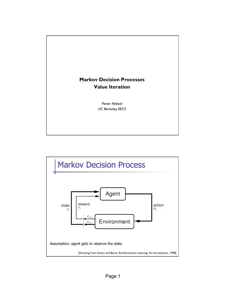
[Drawing from Sutton and Barto, Reinforcement Learning: An Introduction, 1998]

Markov Decision Process

Assumption: agent gets to observe the state

Page 2

Markov Decision Process (S, A, T, R, H)

Given

n

S: set of states

n

A: set of actions

n

T: S x A x S x {0,1,…,H} à [0,1], Tt(s,a,s’) = P(st+1 = s’ | st = s, at =a)

n

R: S x A x S x {0, 1, …, H} à < Rt(s,a,s’) = reward for (st+1 = s’, st = s, at =a)

n

H: horizon over which the agent will act Goal:

n

Find ¼ : S x {0, 1, …, H} à A that maximizes expected sum of rewards, i.e.,

MDP (S, A, T, R, H), goal:

q Cleaning robot q Walking robot q Pole balancing q Games: tetris, backgammon q Server management q Shortest path problems q Model for animals, people

Examples

Page 3

Canonical Example: Grid World

§ The agent lives in a grid § Walls block the agent’s path § The agent’s actions do not always go as planned:

§ 80% of the time, the action North takes the agent North (if there is no wall there) § 10% of the time, North takes the agent West; 10% East § If there is a wall in the direction the agent would have been taken, the agent stays put

§ Big rewards come at the end

Grid Futures

6

Deterministic Grid World Stochastic Grid World

X X

E N S W

X

E N S W ?

X X X

Page 4

Solving MDPs

n In an MDP, we want an optimal policy π*: S x 0:H → A

n A policy π gives an action for each state for each time n An optimal policy maximizes expected sum of rewards n

Contrast: In deterministic, want an optimal plan, or sequence of actions, from start to a goal

t=0 t=1 t=2 t=3 t=4 t=5=H

Value Iteration

n Idea:

n

= the expected sum of rewards accumulated when starting from state s and acting optimally for a horizon of i steps

n Algorithm:

n Start with

for all s.

n For i=1, … , H

Given Vi*, calculate for all states s 2 S:

n This is called a value update or Bellman update/back-up

Page 5

Example Example: Value Iteration

n Information propagates outward from terminal states

and eventually all states have correct value estimates

V2 V3

Page 6

Practice: Computing Actions

n Which action should we chose from state s:

n Given optimal values V*? n = greedy action with respect to V* n = action choice with one step lookahead w.r.t. V* 11

n

Optimal control: provides general computational approach to tackle control problems.

n Dynamic programming / Value iteration

n Discrete state spaces (DONE!) n Discretization of continuous state spaces n Linear systems n LQR n Extensions to nonlinear settings: n Local linearization n Differential dynamic programming

n Optimal Control through Nonlinear Optimization

n Open-loop n Model Predictive Control

n Examples:

Today and forthcoming lectures