SLIDE 1 Markov chain Monte Carlo (MCMC) methods
Gibbs Sampler
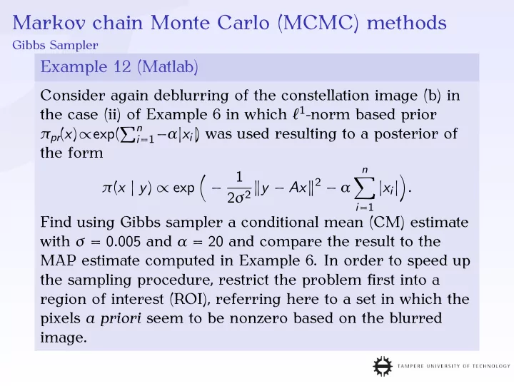
Example 12 (Matlab)
Consider again deblurring of the constellation image (b) in the case (ii) of Example 6 in which ℓ1-norm based prior πpr(x)∝exp(n
i=1−α|xi|
) was used resulting to a posterior of the form π(x | y) ∝ exp
1 2σ2 y − Ax2 − α
n
|xi|
Find using Gibbs sampler a conditional mean (CM) estimate with σ = 0.005 and α = 20 and compare the result to the MAP estimate computed in Example 6. In order to speed up the sampling procedure, restrict the problem first into a region of interest (ROI), referring here to a set in which the pixels a priori seem to be nonzero based on the blurred image.
SLIDE 2
Markov chain Monte Carlo (MCMC) methods
Gibbs Sampler
Example 12 (Matlab) continued
Solution The ROI consisted of seven 7 × 7 pixel sets cocentric with the stars, one set per each star. With the ROI, he dimension of the inverse problem was 73 = 343 and without it 642 = 4096. Exact Blurred ROI
SLIDE 3 Markov chain Monte Carlo (MCMC) methods
Gibbs Sampler
Example 12 (Matlab) continued
The challenge in implementing the Gibbs sampler was mainly in localizing the "essential" part of the conditional posterior density π(xi | y, x1, . . . , xi−1, xi+1, . . . , xn) = π(xi | yi)∝exp
1 2σ2 y − aixi2 − αxi
where ai denotes the i-th column of A = (a1, a2, . . . , an),
j=i ajxj and xi = |xi|, since pixel values must a
priori be positive xi ≥ 0, i = 1, 2, . . . , n. The maximum is located at the point satisfying 0 = d dxi
1 2σ2 yi − aixi2 − αxi
d dxi
1 2σ2 yT
i
yi + 1 σ2 yT
i ai − α
1 2σ2 aT
i aix2 i
SLIDE 4 Markov chain Monte Carlo (MCMC) methods
Gibbs Sampler
Example 12 (Matlab) continued
= −α + 1 σ2 yT
i ai − 1
σ2 aT
i aixi = 0,
i.e. xi = ασ2 − yT
i ai
aT
i ai
, if (ασ2 − yT
i ai)/(aT i ai) > 0, and otherwise the maximizer is
xi = 0. Denoting the maximum value of pi(xi) = − 1 2σ2 yT
i
yi + 1 σ2 yT
i ai − α
1 2σ2 aT
i aix2 i ,
xi ≥ 0 by M, the essential part of the conditional posterior density can be defined as the interval, in which pi(xi) ≥ M − c with some suitably chosen constant c > 0. Since pi(xi) is a second degree polynomial with the second-degree coefficient
SLIDE 5 Markov chain Monte Carlo (MCMC) methods
Gibbs Sampler
Example 12 (Matlab) continued
aT
i ai/(2σ2) and maximizer max{0, (ασ2 −
yT
i ai)/(aT i ai)}, the
interval in which pi(xi) ≥ M − c and xi > 0 is given by Ic =
yT
i ai
aT
i ai
−σ
aT
i ai
yT
i ai
aT
i ai
+σ
aT
i ai
if (ασ2 − yT
i ai)/(aT i ai) > 0, and otherwise this interval is
Ic =
yT
i ai
aT
i ai
+
yT
i ai
aT
i ai
2 + 2σ2c aT
i ai
SLIDE 6 Markov chain Monte Carlo (MCMC) methods
Gibbs Sampler
Example 12 (Matlab) continued
The interval Ic chosen as shown on the previous page contains the maximum value of the conditional posterior density and all the values on the interval are larger or equal to exp(−c) times the maximum. If the constant c is chosen appropriately, then the Gibbs sampler will both be numerically stable and produce unbiased results. Here, the choice was c = 7 and the conditional posterior was evaluated
- n Ic in 20 equally distributed points (examples below).
SLIDE 7
Markov chain Monte Carlo (MCMC) methods
Gibbs Sampler
Example 12 (Matlab) continued
In the sampling process, a total number 10000 sample points were generated first 1000 of which were labeled as the burn-in sequence, which was excluded from the eventual sample enseble yielding the CM estimate. Exact MAP (Example 6) CM
SLIDE 8
Markov chain Monte Carlo (MCMC) methods
Gibbs Sampler
Example 12 (Matlab) continued
The sampling history and sample based marginal density were analyzed for two individual pixels (A) and (B).
(A), History (A), Marginal (A), Burn-in (B), History (B), Marginal (B), Burn-in purple = exact, green = conditional mean, black = 95 % credibility
SLIDE 9 Markov chain Monte Carlo (MCMC) methods
Gibbs Sampler
Example 13 (Matlab)
Consider deblurring of the constellation image in the case of the conditionally gaussian (hierarchical) prior model πpr(x, θ) = π(x | θ)πhyper(θ)
- f Examples 7 and 8. Use the Gibbs sampler to find a
conditional mean (CM) estimate corresponding to both gamma and inverse gamma hyperprior πhyper(θ). Use the noise standard deviation of σ = 0.005 and shape and scaling parameter values β = 1.5 and θ0 = 0.00125 for the gamma and inverse gamma density. Compare the CM estimates
- btained to the corresponding MAP estimates (see,
Examples 6, 7 and 8).
SLIDE 10 Markov chain Monte Carlo (MCMC) methods
Gibbs Sampler
Example 13 (Matlab) continued
Solution The sampling procedure was based on utilizing the conditional posterior densities of the form π(x | y, θ) and π(θ | y, x) according to the following algorithm:
- 1. Choose x(0) and θ(0) and set k = 1.
- 2. Pick x(k) from π(x | y, θ(k−1)).
- 3. Pick θ(k) from π(θ | y, x(k)).
- 4. If k is smaller than the desired number of sampling
points, set k = k + 1 and go back to the second step.
SLIDE 11 Markov chain Monte Carlo (MCMC) methods
Gibbs Sampler
Example 13 (Matlab) continued
The conditional density of the second step is of the form π(x | y, θ(k−1)) ∝ exp
2σ2 y −Ax2− 1 2xTD−1
θ(k−1)x
= exp
2
D−1/2
θ(k−1)
σ−1y
with Dθ(k−1) = diag(θ(k−1)
1
, θ(k−1)
2
, . . . , θ(k−1)
n
). By defining Mθ = σ−1A D−1/2
θ
b = σ−1y
we have π(x | y, θ) ∝ exp(−1
2Mθx − b2) the mean and
covariance matrix of which are given by xθ = (MT
θ Mθ)−1MT θ b
and Γθ = (MT
θ Mθ)−1, respectively.
SLIDE 12 Markov chain Monte Carlo (MCMC) methods
Gibbs Sampler
Example 13 (Matlab) continued
Let now X satisfy the equation Mθ(X − xθ) = Z in the least-squares sense, that is, MT
θ Mθ(X − xθ) = MT θ Z. If Z is
zero-mean Gaussian white noise Z ∼ N(0, I), i.e. E[ZZ T] = I, then X = (MT
θ Mθ)−1MT θ Z + xθ is also Gaussian random
variable with the mean xθ and the covariance matrix E[(X −xθ)(X −xθ)T] = E
θ Mθ)−1MT θ Z
θ Mθ)−1MT θ Z)
T = E
θ Mθ)−1MT θ ZZ TMθ(MT θ Mθ)−1
= (MT
θ Mθ)−1MT θ E[ZZ T]Mθ(MT θ Mθ)−1
= (MT
θ Mθ)−1(MT θ Mθ)(MT θ Mθ)−1
= (MT
θ Mθ)−1 = Γθ,
that is, X ∼ N(xθ, Γθ).
SLIDE 13
Markov chain Monte Carlo (MCMC) methods
Gibbs Sampler
Example 13 (Matlab) continued
Consequently, if z is picked from the zero-mean Gaussian white noise distribution N(0, I), then x = (MT
θ Mθ)−1MT θ z + xθ = (MT θ Mθ)−1MT θ (z + b)
is distributed according to π(x | y, θ). If now z = (z1, z2), then expanding the above equation for θ(k−1) gives the formula x = (σ−2ATA + D−1
θ(k−1))−1(σ−1ATy + σ−1ATz1 + D−1/2 θ(k−1)z2)
= (ATA + σ2D−1
θ(k−1))−1(σATy + σATz1 + σ2D−1/2 θ(k−1)z2),
which was used to pick x(k) from π(x | y, θ(k−1)) on the second step of the sampling procedure.
SLIDE 14 Markov chain Monte Carlo (MCMC) methods
Gibbs Sampler
Example 13 (Matlab) continued
Gibbs sampler was used on the third step to pick θ(k) from π(θ | y, x(k)). If the gamma hyperprior is in question, then π(θ | y, x(k)) ∝ exp
n
x(k)i 2 2θi + θi θ0 − (β − 3 2)log θi
and, again, if the inverse gamma is used, then π(θ | y, x(k)) ∝ exp
n
x(k)
i 2
+ 2θ0 2θi + (β + 3 2)log θi
In both cases, each one-dimensional conditional density is of the form π(θi | y, x(k), θ1, . . . , θi−1, θi+1, . . . , θn) ∝ exp[−fi(θi)]. The essential part of exp[−fi(θi)] was sought by first finding
SLIDE 15
Markov chain Monte Carlo (MCMC) methods
Gibbs Sampler
Example 13 (Matlab) continued
the maximizer θmax
i
satisfying f ′
i (θmax i
) = 0. After that, the quadratic approximation fi(t) ≈ fi(θmax
i
) + f ′
i (θmax i
)(t − θmax
i
) + 1 2f ′′
i (θmax i
)(t − θmax
i
)2 was utilized to estimate the solution of fi(t) = fi(θmax
i
) − c by solving the equation c + f ′
i (θmax i
)(t − θmax
i
) + 1 2f ′′
i (θmax i
)(t − θmax
i
)2 = 0. The solution t was then chosen as the initial iterate t[0] to Newton’s iteration t[ℓ] = t[ℓ−1] − [f (t[ℓ−1]) − fi(θmax
i
) + c]/f ′(t[ℓ−1]).
SLIDE 16 Markov chain Monte Carlo (MCMC) methods
Gibbs Sampler
Example 13 (Matlab) continued
The third iterate t[3] was used as the final estimate. The interval Ic = [ε, t[3]], where ε = 2.2204 · 10−16, was used to approximate the (essential) support of exp[−fi(θi)]. This density was evaluated in 20 points equally spaced on Ic with c = 7 (see the figures below). A total number 10000 sample points were generated first 1000 of which were labeled as the burn-in sequence excluded from the eventual sample enseble.
Gamma
SLIDE 17
Markov chain Monte Carlo (MCMC) methods
Gibbs Sampler
Example 13 (Matlab) continued
Gamma Hyperprior Exact MAP (Example 6) CM
SLIDE 18
Markov chain Monte Carlo (MCMC) methods
Gibbs Sampler
Example 13 (Matlab) continued
Gamma Hyperprior (A), History (A), Marginal (A), Burn-in (B), History (B), Marginal (B), Burn-in
SLIDE 19
Markov chain Monte Carlo (MCMC) methods
Gibbs Sampler
Example 13 (Matlab) continued
Inverse Gamma Hyperprior Exact MAP (Example 7) CM
SLIDE 20
Markov chain Monte Carlo (MCMC) methods
Gibbs Sampler
Example 13 (Matlab) continued
Inverse Gamma Hyperprior (A), History (A), Marginal (A), Burn-in (B), History (B), Marginal (B), Burn-in
SLIDE 21
Markov chain Monte Carlo (MCMC) methods
Gibbs Sampler
Example 14 (Matlab)
Compare the MAP and CM estimates of Ex. 6, 7, 12, and 13. Solution
Exact MAP, ℓ1 MAP, Gamma MAP, Inv. G. Exact CM, ℓ1 CM, Gamma CM, Inv. G.